Inverse theory exists to make the life of the mantle geodynamicist easier.
The Geodynamics 101 series serves to showcase the diversity of research topics and methods in the geodynamics community in an understandable manner. We welcome all researchers – PhD students to professors – to introduce their area of expertise in a lighthearted, entertaining manner and touch upon some of the outstanding questions and problems related to their fields. This time, Lars Gebraad, PhD student in seismology at ETH Zürich, Switzerland, talks about inversion and how it can be used in geodynamics! Due to the ambitious scope of this topic, we have a 3-part series on this! You can find the first post here. This week, we have our final post in the series, where Lars discusses probabilistic inversion.
 One integral part of doing estimations on parameters is an uncertainty analysis. The aim of a general inverse problem is to find the value of a parameter, but it is often very helpful to indicate the measure of certainty. For example in the last figure of my previous post, the measurement values at the surface are more strongly correlated to the upper most blocks. Therefore, the result of an inversion in this set up will most likely be more accurate for these parameters, compared to the bottom blocks.
In linear deterministic inversion, the eigenvalues of the matrix system provide an indication of the resolvability of parameters (as discussed in the aforementioned work by Andrew Curtis). There are classes of methods to compute exact parameter uncertainty in the solution.
From what I know, for non-linear models, uncertainty analysis is limited to the computation of second derivatives of the misfit functional in parameter space. The second derivatives of X (the misfit function) are directly related to the standard deviations of the parameters. Thus, by computing all the second derivatives of X, a non-linear inverse problem can still be interrogated for its uncertainty. However, the problem with this is its linearisation; linearising the model and computing derivatives may not be truly how the model reacts in model space. Also, for strongly non-linear models many trade-offs (correlations) exist which influence the final solution, and these correlations may very strongly depending on the model to be inverted.
Bayes’ rule
Enter reverend Thomas Bayes
This part-time mathematician (he only ever published one mathematical work) from the 18th century formulated the Bayes’ Theorem for the first time, which combines knowledge on parameters. The mathematics behind it can be easily retrieved from our most beloved/hated Wikipedia, so I can avoid getting to caught up in it. What is important is that it allows us to combine two misfit functions or probabilities. Misfits and probabilities are directly interchangeable; a high probability of a model fitting our observations corresponds to a low misfit (and there are actual formulas linking the two). Combining two misfits allows us to accurately combine our pre-existing (or commonly: prior) knowledge on the Earth with the results of an experiment. The benefits of this are two-fold: we can use arbitrarily complex prior knowledge and by using prior knowledge that is bounded (in parameter space) we can still invert underdetermined problems without extra regularisation. In fact, the prior knowledge acts as regularisation.
One probabilistic regularised bread, please
Let’s give our friend Bayes a shot at our non-linear 1D bread. We have to come up with our prior knowledge of the bread, and because we did not need that before I’m just going to conjure something up! We suddenly find the remains of a packaging of 500 grams of flour
This is turning in quite the detective story!
However, the kitchen counter that has been worked on is also royally covered in flour. Therefore, we estimate that probably this pack was used; about 400 grams of it, with an uncertainty (standard deviation) of 25 grams. Mathematically we can formulate our prior knowledge as a Gaussian distribution with the aforementioned standard deviation and combine this with our misfit of the inverse problem (often called the likelihood). The result is given here:
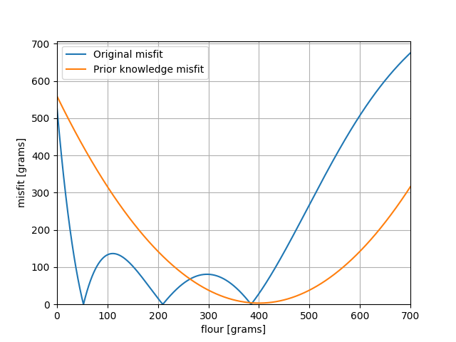
Prior and original misfit

Combined misfit
One success and one failure!
First, we successfully combined the two pieces of information to make an inverse problem that is no longer non-unique (which was a happy coincidence of the prior: it is not guaranteed). However, we failed to make the problem more tractable in terms of computational requirements. To get the result of our combined misfit, we still have to do a systematic grid search, or at least arrive at a (local) minimum using gradient descent methods.
We can do the same in 2D. We combine our likelihood (original inverse problem) with rather exotic prior information, an annulus in model space, to illustrate the power of Bayes’ theorem. The used misfit functions and results are shown here:
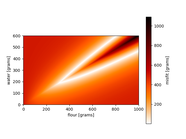
Original misfit for a bread of 500 grams
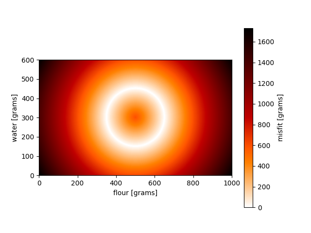
Prior knowledge misfit

Combined misfit
This might also illustrate the need for non-linear uncertainty analysis. Trade-offs at the maxima in model space (last figure, at the intersection of the circle and lines) distinctly show two correlation directions, which might not be fully accounted for by using only second derivative approximations.
Despite this ‘non-progress’ of still requiring a grid search even after applying probability theory, we can go one step further by combining the application of Bayesian inference with the expertise of other fields in appraising inference problems…
Jump around!
Up to now, using a probabilistic (Bayesian) approach has only (apparently) made our life more difficult! Instead of one function, we now have to perform a grid search over the prior and the original problem. That doesn’t seem like a good deal. However, a much used technique in statistics deals with exactly the kind of problems we are facing here: given a very irregular and high dimensional function
How do we extract interesting information (preferably without completely blowing our budget on supercomputers)?
Let’s first say that with interesting information I mean minima (not necessarily restricted to global minima), correlations, and possibly other statistical properties (for our uncertainty analysis). One answer to this question was first applied in Los Alamos around 1950. The researches at the famous institute developed a method to simulate equations of state, which has become known as the Metropolis-Hastings algorithm. The algorithm is able to draw samples from a complicated probability distribution. It became part of a class of methods called Markov Chain Monte Carlo (MCMC) methods, which are often referred to as samplers (technically they would be a subset of all available samplers).
The reason that the Metropolis-Hastings algorithm (and MCMC algorithms in general) is useful, is that a complicated distribution (e.g. the annulus such as in our last figure) does not easily allow us to generate points proportional to its misfit. These methods overcome this difficulty by starting at a certain point in model space and traversing a random path through it – jumping around – but visiting regions only proportional to the misfit. So far, we have only considered directly finding optima to misfit functions, but by generating samples from a probability distribution proportional to the misfit functions, we can readily compute these minima by calculating statistical modes. Uncertainty analysis subsequently comes virtually for free, as we can calculate any statistical property from the sample set.
I won’t try to illustrate any particular MCMC sampler in detail. Nowadays many great tools for visualising MCMC samplers exist. This blog by Alex Rogozhnikov does a beautiful job of both introducing MCMC methods (in general, not just for inversion) and illustrating the Metropolis Hastings Random Walk algorithm as well as the Hamiltonian Monte Carlo algorithm. Hamiltonian Monte Carlo also incorporates gradients of the misfit function, thereby even accelerating the MCMC sampling. Another great tool is this applet by Chi Feng. Different target distributions (misfit functions) can be sampled here by different algorithms.
The field of geophysics has been using these methods for quite some time (Malcom Sambridge writes in 2002 in a very interesting read that the first uses were 30 years ago), but they are becoming increasingly popular. However, strongly non-linear inversions and big numerical simulations are still very expensive to treat probabilistically, and success in inverting such a problem is strongly dependent on the appropriate choice of MCMC sampler.
Summary of probabilistic inversions
In the third part of this blog we saw how to combine any non-linear statistical model, and how to sample these complex functions using MCMC samplers. The resulting sample sets can be used to do an inversion and compute statistical moments of the inverse problem.
Some final thoughts
If you reached this point while reading most of the text, you have very impressively worked your way through a huge amount of inverse theory! Inverse theory is a very diverse and large field, with many ways of approaching a problem. What’s discussed here is, to my knowledge, only a subset of what’s being used ‘in the wild’. These ramblings of a aspiring seismologist might sound uninteresting to the geodynamiscists at the other side of the geophysics field. Inverse methods seem to be not nearly discussed as much in geodynamics as they are in seismology. Maybe it’s the terminology that differs, and that all these concepts are well known and studied under different names and you recognise some of the methods. Otherwise, I hope I have given an insight in the wonderful and sometimes ludicrous mathematical world of (some) seismologists.
Interested in playing around with inversion yourself? You can find a toy code about baking bread here.