the Creative Commons Attribution 4.0 License.
the Creative Commons Attribution 4.0 License.
 | 23 Apr 2020
Intercomparison of wind observations from the European Space Agency's Aeolus satellite mission and the ALADIN Airborne Demonstrator
Christian Lemmerz
Fabian Weiler
Uwe Marksteiner
Benjamin Witschas
Stephan Rahm
Alexander Geiß
Oliver Reitebuch
Shortly after the successful launch of the European Space Agency's wind mission Aeolus, co-located airborne wind lidar observations were performed in central Europe; these observations employed a prototype of the satellite instrument – the ALADIN (Atmospheric LAser Doppler INstrument) Airborne Demonstrator (A2D). Like the direct-detection Doppler wind lidar on-board Aeolus, the A2D is composed of a frequency-stabilized ultra-violet (UV) laser, a Cassegrain telescope and a dual-channel receiver to measure line-of-sight (LOS) wind speeds by analysing both Mie and Rayleigh backscatter signals. In the framework of the first airborne validation campaign after the launch and still during the commissioning phase of the mission, four coordinated flights along the satellite swath were conducted in late autumn of 2018, yielding wind data in the troposphere with high coverage of the Rayleigh channel. Owing to the different measurement grids and LOS viewing directions of the satellite and the airborne instrument, intercomparison with the Aeolus wind product requires adequate averaging as well as conversion of the measured A2D LOS wind speeds to the satellite LOS (LOS*). The statistical comparison of the two instruments shows a positive bias (of 2.6 m s−1) of the Aeolus Rayleigh winds (measured along its LOS*) with respect to the A2D Rayleigh winds as well as a standard deviation of 3.6 m s−1. Considering the accuracy and precision of the A2D wind data, which were determined from comparison with a highly accurate coherent wind lidar as well as with the European Centre for Medium-Range Weather Forecasts (ECMWF) model winds, the systematic and random errors of the Aeolus LOS* Rayleigh winds are 1.7 and 2.5 m s−1 respectively. The paper also discusses the influence of different threshold parameters implemented in the comparison algorithm as well as an optimization of the A2D vertical sampling to be used in forthcoming validation campaigns.


On 22 August 2018, the fifth Earth Explorer mission of the European Space Agency (ESA) – Aeolus – was launched into space, marking an important milestone in the centennial history of atmospheric observing systems (Stith et al., 2018; Kanitz et al., 2019; Reitebuch et al., 2019; Straume et al., 2019). Aeolus is the first mission to acquire atmospheric wind profiles from the ground to the lower stratosphere on a global scale, and it deploys the first-ever satellite-borne wind lidar system ALADIN (Atmospheric LAser Doppler INstrument; ESA, 2008; Stoffelen et al., 2005; Reitebuch, 2012). Circling the Earth on a sun-synchronous orbit with a repeat cycle of 1 week, ALADIN provides one component of the wind vector along the instrument's line of sight (LOS) from the ground up to an altitude of 30 km with a vertical resolution of 0.25 to 2 km depending on altitude. The near-real-time wind observations from Aeolus contribute to improving the accuracy of numerical weather prediction (Isaksen and Rennie, 2019; Rennie and Isaksen, 2019a, b) and advancing the understanding of atmospheric dynamics and processes relevant to climate variability. In particular, wind profiles acquired in the tropics and over the oceans help to close large gaps in the global wind data coverage which, before the launch of Aeolus, represented a major deficiency in the Global Observing System (Baker et al., 2014; Andersson, 2018; NAS, 2018). In addition to the wind data product, Aeolus provides information on cloud top heights and on the vertical distribution of aerosol and cloud properties, such as backscatter and extinction coefficients (Flamant et al., 2008; Ansmann et al., 2007).
Several years before the launch of the fifth Earth Explorer mission, an airborne prototype of the Aeolus payload – the ALADIN Airborne Demonstrator (A2D) – was developed at the German Aerospace Center (Deutsches Zentrum für Luft- und Raumfahrt e.V.; DLR). Due to its representative design and operating principle, the A2D has since delivered valuable information on the wind measurement strategies of the satellite instrument as well as on the optimization of the wind retrieval and related quality control algorithms. Broad vertical and horizontal coverage across the troposphere is achieved due to the complementary design of the A2D receiver which, like ALADIN, comprises a Rayleigh and a Mie channel for analysing both molecular and particulate backscatter signals. In addition to the A2D, a well-established coherent Doppler wind lidar (2 µm DWL) has been operated at DLR for many years. As it is equipped with a double-wedge scanner, the 2 µm DWL allows for the determination of the wind vector with high accuracy and precision (Weissmann et al., 2005; Chouza et al., 2016; Witschas et al., 2017). Thus, both wind lidar systems represent key instruments for the calibration and validation (Cal/Val) activities during the Aeolus mission.
Over the past few years, both systems have been deployed in several field experiments for the purpose of prelaunch validation of the satellite instrument and of performing wind lidar observations under various atmospheric conditions (Marksteiner et al., 2018; Lux et al., 2018). In autumn of 2018, the first airborne campaign following the launch of Aeolus was carried out from the Oberpfaffenhofen airbase, Germany. Aside from extending the existing data set of wind observations, this field experiment aimed to perform several underflights of Aeolus in central Europe in order to provide first comparative wind results between the A2D and the satellite instrument during its commissioning phase. Moreover, the campaign had the objective of optimizing the operational procedures, particularly in terms of flight planning, that will be applied during the forthcoming Cal/Val campaigns in the operational phase of Aeolus.
This paper presents the results from the first airborne validation campaign of the Aeolus mission and demonstrates the methodology used to compare the different data sets from the A2D and the satellite instrument. In this context, it intends to serve as a reference for later studies related to the airborne validation of Aeolus. More specifically, this work shows how to account for the different LOS directions in order to make the wind data sets comparable. This procedure is not only required for the A2D but also for any other Cal/Val instrument that measures only one component of the wind vector, such as the LEANDRE New Generation (LNG; Bruneau et al., 2015) that is also foreseen to be deployed on airborne campaigns for Aeolus validation.
The text is organized as follows. First, the designs and operation principles of ALADIN and the A2D are briefly described with a focus on the commonalities and differences of the two wind lidar instruments (Sect. 2). Section 3 gives an overview of the validation campaign including the flight planning procedures and the A2D calibration. The wind observations from the research flight along the satellite swath performed on 22 November 2018 are also presented in this section (Sect. 3.2, 3.3), followed by an assessment of the A2D wind data accuracy and precision by means of the 2 µm coherent wind lidar (Sect. 3.4). In Sect. 4, the adaptation of the A2D wind data to the Aeolus measurement grid and viewing geometry is explained (Sect. 4.1, 4.2), which is prerequisite for the subsequent comparison of the two data sets with model wind data from the ECMWF (Sect. 4.3) and with each other (Sect. 4.4). The influence of two selected threshold parameters incorporated in the comparison algorithm on the outcome of the statistical comparison is also discussed (Sect. 4.5). Due to the sparse coverage of Mie wind data gained during the campaign, the analysis is restricted to the A2D and Aeolus Rayleigh channels. The comparison of the 2 µm DWL wind data with those of Aeolus is the subject of another publication (Witschas et al., 2020). Finally, an optimized range gate setting of the A2D is proposed that aims to improve the validation capabilities of the instrument in forthcoming airborne campaigns that are to be conducted during the Aeolus mission (Sect. 4.6).
The single payload of the Aeolus satellite, ALADIN, represents one of the most sophisticated Earth observation instruments ever put into orbit. While it has only been operating in space since its launch in August 2018, the A2D has been employed on the ground and in research flights since 2005. The designs and measurement principles of the two direct-detection Doppler wind lidars have been extensively specified in previous publications that have described the satellite (ESA, 2008; Stoffelen et al., 2005; Reitebuch, 2012; Kanitz et al., 2019) and airborne (Reitebuch et al., 2009; Paffrath et al., 2009; Lux et al., 2018) instruments respectively. Therefore, only a brief description of the A2D is presented in this work, followed by a short explanation of the Aeolus wind data product that is validated later in the text.
2.1 The A2D direct-detection wind lidar system
A simplified schematic of the airborne instrument is illustrated in Fig. 1. Like ALADIN, the system consists of a pulsed, frequency-stabilized, ultra-violet (UV) laser transmitter, a Cassegrain-type telescope, a configuration to combine a fraction of the emitted radiation with the atmospheric and ground return signals (front optics), and a dual-channel receiver including detectors.
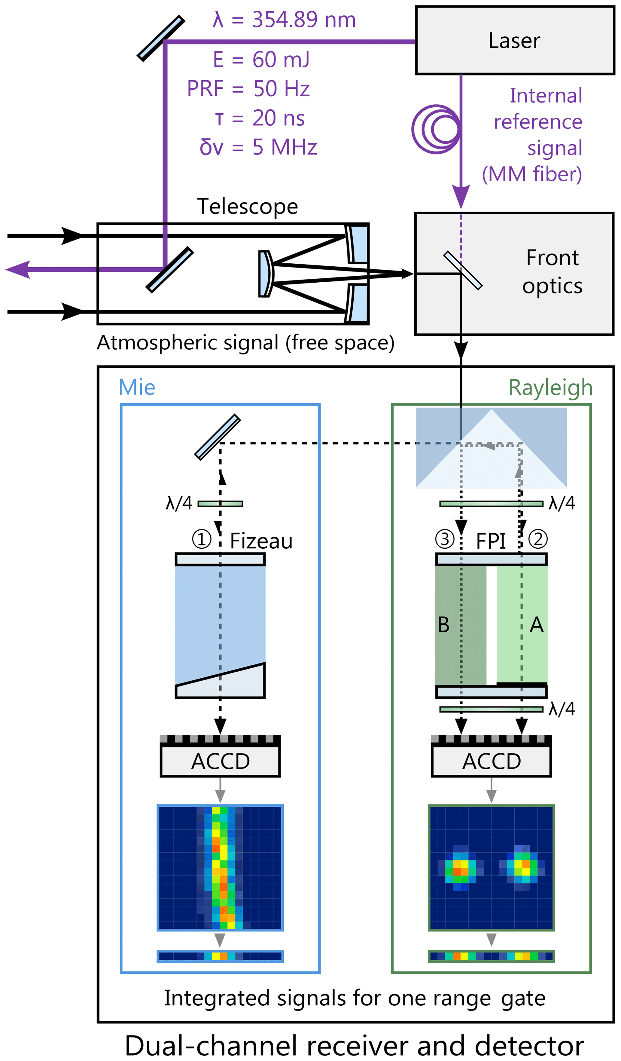
Figure 1Schematic of the ALADIN Airborne Demonstrator (A2D) wind lidar instrument consisting of a frequency-stabilized, ultra-violet laser transmitter, a Cassegrain telescope, front optics and a dual-channel receiver. The latter is composed of a Fizeau interferometer and sequential Fabry–Pérot interferometers (FPI) for analysing the Doppler frequency shift from particulate and molecular backscatter signals respectively. PRF refers to the pulse repetition frequency, MM stands for multimode and ACCD refers to the accumulation charge-coupled device.
The laser transmitter is realized by a frequency-tripled Nd:YAG master oscillator power amplifier (MOPA) system that generates UV laser pulses at 354.89 nm wavelength with a duration of 20 ns (full width at half maximum, FWHM) and an energy of 60 mJ at 50 Hz repetition rate (3.0 W average power). Injection-seeding of the master oscillator in combination with an active frequency-stabilization technique (Lemmerz et al., 2017) provides single-frequency operation with a pulse-to-pulse frequency stability of approximately 3 MHz (rms) and a spectral bandwidth of 50 MHz (FWHM). The near-diffraction-limited beam (beam quality factor: M2 < 1.3) is transmitted to the atmosphere via a piezoelectrically controlled mirror that is attached to the frame of a telescope in Cassegrain configuration. In contrast to the satellite instrument that uses a 1.5 m diameter telescope in transceiver configuration and operates at an off-nadir viewing angle of 35∘, the A2D incorporates a 0.2 m diameter telescope that is oriented at an off-nadir angle of 20∘. Owing to the structural design of the telescope, a range-dependent overlap function has to be considered in the wind retrieval, as described in Paffrath et al. (2009).
The backscattered radiation from the atmosphere and the ground is collected by the convex spherical secondary mirror of the telescope and directed to the front optics of the A2D receiver assembly. After passing through a narrowband UV bandpass filter (FWHM: 1.0 nm) that blocks the broadband solar background spectrum, the return signal is spatially overlapped with a small portion of the outgoing laser radiation which is referred to as internal reference signal. The latter is analysed to determine the transmitted laser frequency before the atmospheric return and to calibrate the frequency-dependent transmission of the receiver spectrometers, which are required for accurate wind retrieval. Unlike Aeolus where the internal reference signal is guided to the front optics on a free optical path, a multimode fibre (200 µm core diameter) is employed in the A2D. Utilization of the multimode fibre introduces detrimental speckle noise that affects the precision of the internal reference frequency determination, as explained in Lux et al. (2018). Hence, a fibre scrambler was recently integrated between the laser transmitter and the front optics in order to reduce the speckle noise and, in turn, to significantly improve the stability of the internal reference frequency and signal intensity (Lux et al., 2019).
The design of the A2D receiver is almost identical to that of the satellite instrument: it comprises two complementary channels to separately analyse the return signals from both molecules (Rayleigh channel) and particles like clouds and aerosols (Mie channel); see the lower part of Fig. 1. A Fizeau interferometer is used to measure the Doppler frequency shift of the narrowband Mie signal (FWHM ≈50 MHz) that originates from cloud and aerosol backscattering, while two sequential Fabry–Pérot interferometers (FPIs) are employed to determine the Doppler shift of the broadband Rayleigh backscatter signal from molecules (FWHM ≈3.8 GHz at 355 nm and 293 K). The Mie channel is based on the fringe-imaging technique (McKay, 2002), which relies on the measurement of the spatial location of a linear interference pattern (fringe) that is vertically imaged onto the detector. A Doppler frequency shift of the return signal (where f0=844.75 THz is the laser emission frequency, and c is the speed of light) manifests as a spatial displacement of the fringe centroid position with an approximately linear relationship for typical wind speeds vLOS along the laser beam LOS well below 100 m s−1 (ΔfDoppler < 563 MHz).
Due to the much broader spectral bandwidth of the molecular backscatter signal that features a Rayleigh–Brillouin line shape (Witschas et al., 2010; Witschas, 2011a, b), a different technique is applied for deriving the Doppler frequency shift in the Rayleigh channel. Here, the measurement principle is based on the double-edge technique (Chanin et al., 1989; Garnier and Chanin, 1992; Flesia and Korb, 1999; Gentry et al., 2000) involving two bandpass filters (A and B) that are realized by the sequential FPIs. Measurement of the contrast between the signals transmitted through the two filters allows for the determination of the frequency shift between the emitted and backscattered laser pulse.
Detection of the Mie and Rayleigh signals is carried out by two accumulation charge-coupled devices (ACCDs) with an array size of 16 pixels×16 pixels (image zone) and a high quantum efficiency of 85 % at 355 nm. For both channels, the electronic charges of all 16 rows in the image zone are binned together to one row and stored in 25 rows of a memory zone, with each row representing one range gate. From the 25 range gates, three range gates are used for detecting the background light, signals resulting from the voltage at the analogue-to-digital converter (detection chain offset, DCO) and the internal reference signal respectively. Two following range gates act as buffers for the internal reference, so that atmospheric backscatter signals are collected in the remaining 20 range gates. Due to the transfer time from the image to the memory zone, the temporal resolution of one range gate is limited to 2.1 µs, which corresponds to a minimum range resolution of 315 m (a height resolution of 296 m considering the 20∘ off-nadir viewing angle of the instrument). The timing sequences of both ACCDs are flexibly programmable so that the vertical resolution within one wind profile can be varied from 296 m to about 1.2 km (individually for the Mie and Rayleigh channels). The horizontal resolution of the A2D is determined by the acquisition time of the detection unit where the signals from 18 successive laser pulses are accumulated to so-called “measurements” (duration 0.4 s). Summation of the signals obtained from 35 measurements, i.e. 630 laser pulses, forms one “observation” (duration 14 s). Considering the time required for data read out and transfer (4 s), two subsequent observations are separated by 18 s.
For the satellite instrument, one observation consists of 30 accumulations (also referred to as measurements) of 19 shots, whereby data are continuously read out without gaps of 4 s. Hence, one observation takes 12 s. However, due to the much higher ground speed of Aeolus (about 7200 m s−1) compared with the Falcon aircraft (200 m s−1), the Aeolus horizontal resolution of about 86.4 km per observation is much coarser than that of the A2D (3.6 km). In the course of the Aeolus wind retrieval, different accumulation lengths are possible depending on the signal strength in the Rayleigh and Mie channels, as explained in the next section.

2.2 The Aeolus wind data product
ALADIN on-board Aeolus is, like the A2D, a direct-detection Doppler wind lidar that incorporates a frequency-stabilized UV laser and a dual-channel optical receiver to determine the Doppler shift from the broadband Rayleigh–Brillouin backscatter from molecules and the narrowband Mie backscatter from aerosols and cloud particles (ESA, 2008; Reitebuch, 2012). The major technical differences to the airborne instrument are the larger telescope diameter (1.5 m), the larger slant angle (35∘) and the free-path propagation of the internal reference signal, as explained above. An overview of the key instrument parameters of the two wind lidars is given in Table 1.
The Aeolus Level 2B (L2B) product contains so-called horizontal line-of-sight (HLOS) winds for the Mie and Rayleigh channel. The L1B and L2B wind retrieval are described in detail in the Algorithm Theoretical Basis Documents (Reitebuch et al., 2018; Tan et al., 2017). Thus, only a brief description is provided here. As a first step, Aeolus measurements (with a horizontal resolution of about 2.9 km corresponding to 0.4 s) are gathered together into groups where the length depends on the L2B parameter settings. During the November 2018 analysis period, the group length was set to 30 Aeolus measurements and was therefore identical to the previously defined observation length (corresponding to a horizontal extent of about 86.4 km). Note that groups can also be shorter than observations if the horizontal averaging is set differently in the L2B processor. The measurement bins within the group are then classified into “clear” and “cloudy” bins using estimates of the backscatter ratio, which is defined as the ratio of the total backscatter coefficient (particles and molecules) to the molecular backscatter coefficient. “Clear” bins are usually those for which the backscatter ratio is below 1.2 to 1.4, depending on L2B processor settings, whereas bins with higher backscatter ratios are considered “cloudy”. Before the wind retrieval is performed, the signals of the measurement bins from the same category are horizontally accumulated within the group. Separate wind retrievals are performed for both channels and for both categories, whereby only Rayleigh winds classified as clear and Mie winds classified as cloudy are generally used for further analysis. In this manner, it is ensured that systematic errors introduced to the Rayleigh winds due to contamination from particulate backscatter signals as well as the low signal-to-noise ratio (SNR) of the Mie channel are avoided. Finally, to account for pressure and temperature effects in the Rayleigh wind retrieval (Dabas et al., 2008), a priori temperature and pressure information from ECMWF model results are interpolated along the Aeolus measurement track and used for correction. The meteorological data utilized are also included in an auxiliary data product (AUX_MET). It should be mentioned that the Aeolus wind data obtained from the L2B product, which is discussed here, are in a preliminary state, inasmuch as biases related to known error sources such as instrumental drifts have not been corrected yet (Reitebuch et al., 2019; Rennie and Isaksen, 2019a). These error sources will be elaborated on in section 4.3.
In addition to the L2B wind product, Aeolus provides an L2C wind product that results from the background assimilation of the Aeolus HLOS winds in the ECMWF operational prediction model. It contains the u and v components of the wind vector and supplementary geophysical parameters. Note that, at the time of the WindVal III campaign, the Aeolus data assimilation was not yet established, which means that the L2C product used in this study contains pure model data along the satellite track.
Only 3 months after the successful launch of Aeolus, the WindVal III wind validation campaign was conducted from the DLR airbase in Oberpfaffenhofen, Germany, in the time frame from 5 November to 5 December 2018. The campaign represented a continuation of the previous field experiments WindVal I in 2015 (Marksteiner et al., 2018) and WindVal II (NAWDEX) in 2016 (Schäfler et al., 2018; Lux et al., 2018) that were performed from Keflavík, Iceland. The previous campaigns aimed at the prelaunch validation of the Aeolus mission, exploiting the high degree of commonality of the A2D with the satellite instrument to test its measurement principle and to refine its wind retrieval algorithms based on real atmospheric measurements. With Aeolus operating in space, the objectives of WindVal III went beyond those of the preceding campaigns. For the first time, co-located wind measurements of ALADIN and the A2D could be performed, providing the possibility to compare the performance of both instruments under various atmospheric conditions. In addition to the co-located wind observations shortly after launch, one goal of the WindVal III campaign was to rehearse the validation activities that will be performed after the commissioning phase of the Aeolus mission. This included, first and foremost, the planning of the flights along the satellite measurement track, which required thorough consideration of the weather conditions along the swath within the reach of the DLR Falcon research aircraft, air traffic control limitations, and the satellite status. For the purpose of high wind data coverage of Aeolus, target areas without high- or mid-level clouds were generally preferred for the underflights. Ideally, the flights included sections with cloud-free conditions, as this allowed for strong ground return signals that could be exploited to reduce potential wind biases by means of zero wind correction (Marksteiner, 2013; Lux et al., 2018).
Table 2Overview of the research flights of the Falcon aircraft in the frame of the WindVal III campaign, and the wind scenes performed with the A2D along the Aeolus measurement track. The A2D was not operable during the flight on 17 November 2018. The wind scene printed in bold is comprehensively discussed in the later sections.
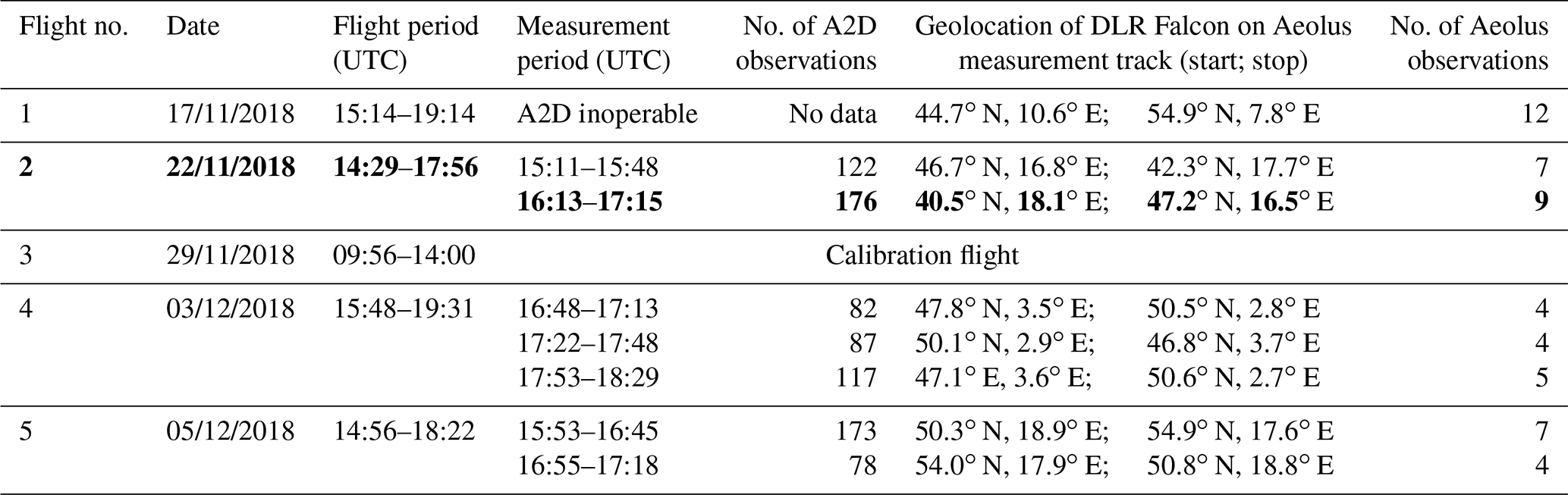
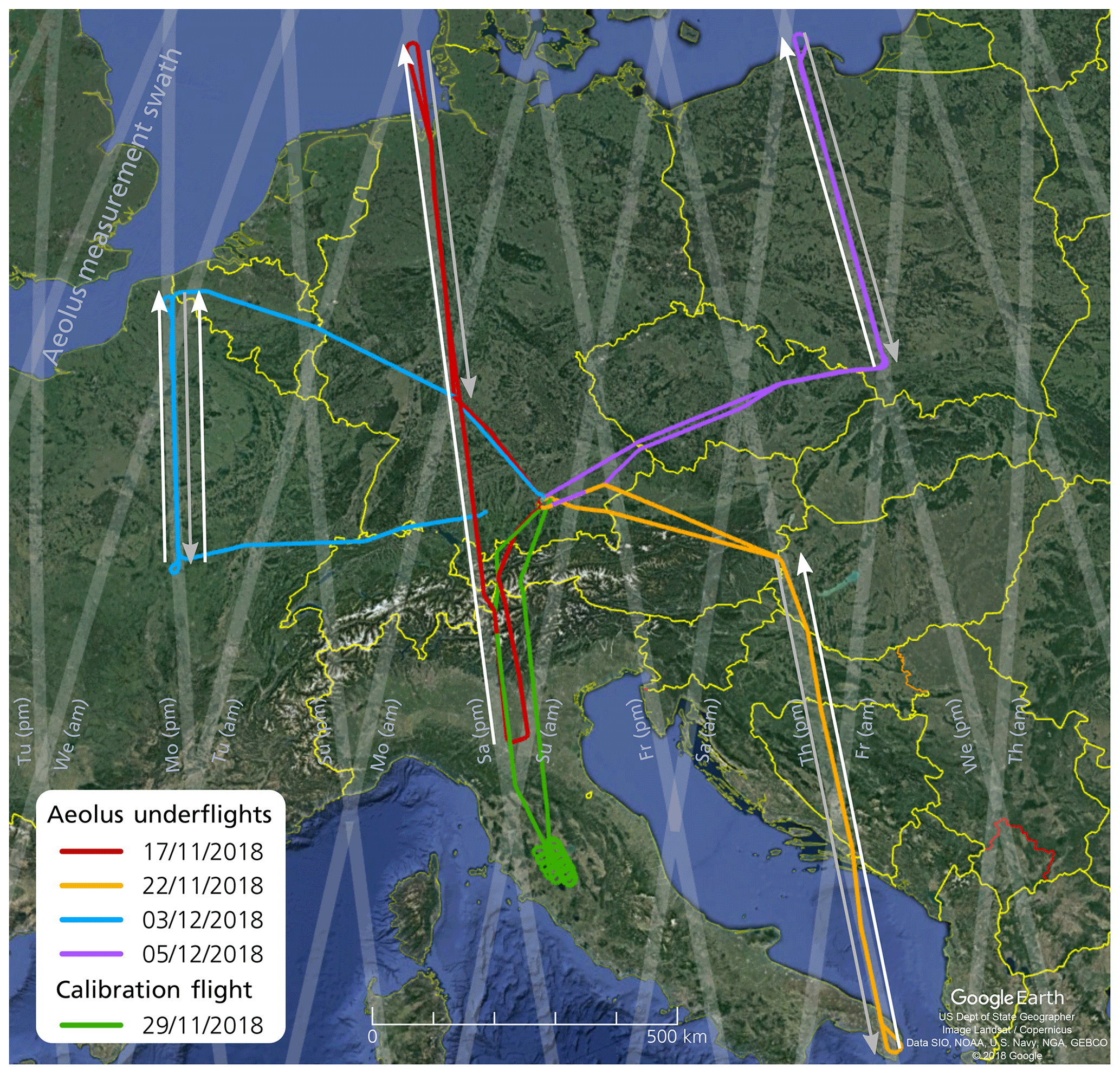
Figure 2Flight tracks of the Falcon aircraft during the WindVal III campaign from 17 November to 5 December 2018 (background image: © 2018 Google). Each colour represents a single flight. The Aeolus measurement swath is shown in grey. The arrows indicate the Falcon flight direction along the swath on the different legs in (white arrows) and against (grey arrows) the satellite direction, which was always from south to north during the probed evening satellite ascending orbits. The A2D was not operated during the flight on 17 November 2018.
In the framework of the WindVal III campaign in autumn 2018, six flights were conducted, including a test flight and a calibration flight. The corresponding flight tracks of the DLR Falcon aircraft and the swaths of the Aeolus satellite for 1 week are shown in Fig. 2. A total of 22 flight hours were carried out, including the test flight performed a few hours before the first underflight on 17 November 2018. Adding up the lengths of the satellite swaths covered by the aircraft during the four underflights, the overall track length for which wind data were acquired for validation purposes was nearly 3000 km. The first underflight was also the longest flight along the Aeolus track (1155 km), covering the measurement swath from northern Italy up to the North Frisian Islands. While the 2 µm DWL was operating without limitations during the entire campaign, the A2D was not operational during the first flight due to technical issues; therefore, A2D wind data are only available from the three other underflights. The data obtained along the Aeolus track were subdivided into seven wind scenes that correspond to the flight legs indicated by arrows in Fig. 2. An overview of these scenes, including the number of A2D observations, is presented in Table 2 along with the geolocations of the start and end points of the respective flight legs. The number of Aeolus observations for each scene is also provided.
3.1 Response calibrations
The flight on 29 November 2018 was dedicated to the calibration of the A2D; this is a prerequisite for the wind retrieval, as the relationship between the Doppler frequency shift of the backscattered light, i.e. the wind speed, and the response of the two spectrometers has to be known for the wind retrieval. Calibration of the Rayleigh and Mie channels involves a frequency scan of the laser transmitter over 1.4 GHz (±125 m s−1) to simulate well-defined Doppler shifts of the atmospheric backscatter signal within the limits of the laser frequency stability. During this procedure, the contribution of (real) wind related to molecular or particular motion along the instruments' LOS is virtually eliminated by flying curves at a 20∘ roll angle of the Falcon aircraft, thereby resulting in approximate nadir viewing angle of the instrument and, for negligible vertical wind, removing LOS wind speed. In the course of one frequency scan, which takes about 24 min, unknown contributions to the Rayleigh and Mie response such as temperature variations of the spectrometers or frequency fluctuations of the laser transmitter have to be minimized, as they can introduce systematic errors or increase the random error of the derived wind speed. Above all, cloud- and aerosol-free conditions are necessary to avoid Mie backscatter signals that affect the backscatter spectrum and, thus, contaminate the Rayleigh response in the respective range gates. Furthermore, ground visibility is required to calibrate the Mie channel. Additional information on the A2D calibration procedure and how it compares to the satellite mission are comprehensively described in Marksteiner et al. (2018), whereas details on the calibration and wind retrieval of Aeolus can be found in Tan et al. (2016) and Reitebuch et al. (2018).
The region between Rome and Florence with clear atmosphere and nearly zero vertical wind was chosen for the WindVal III calibration flight on 29 November 2018. The green track in Fig. 2 shows the characteristic circular flight pattern in northern Italy that follows from the 20∘ roll angle of the aircraft that was undertaken to establish nadir viewing angle of the A2D. In the period from 10:48 to 12:51 UTC, four response calibrations, i.e. laser frequency scans, were performed to obtain four sets of calibration parameters. Based on several quality criteria which were identified during previous campaigns and are mostly related to instrument housekeeping data (Marksteiner et al., 2018), one of the four calibration sets was selected for Rayleigh and Mie wind retrieval respectively. The chosen Rayleigh calibration was especially characterized by high pointing stability of the laser transmitter; this is of high importance for assuring a low random error of the Rayleigh channel, as even small variations in the incidence angle on the Rayleigh FPIs (by a few µrad) largely influence the Rayleigh response, potentially leading to wind errors of several metres per second (DLR, 2016). Moreover, the selected calibration showed the smallest residuals of the fifth-order polynomial fit applied to Rayleigh response curve, thereby ensuring the lowest random wind error, which may result from discrepancies between the calibration fit function and the actual frequency dependence of the spectrometer response. For the Mie channel, the four calibration results were very consistent, which can be traced back to the integration of the fibre scrambler that considerably reduced the speckle noise of the internal reference signal (Lux et al., 2019). Therefore, as there were no additional arguments in favour or against a certain calibration, the one with the lowest temperature variability of the Fizeau interferometer was selected for the Mie wind retrieval.
3.2 A2D wind results from the underflight on 22 November 2018
First, co-located wind observations of the A2D and Aeolus were performed on 22 November when the Falcon flew along the satellite swath from Lecce in southern Italy (40.5∘ N, 18.1∘ E) to the Austrian–Hungarian border (47.2∘ N, 16.5∘ E; see Fig. 2). Aeolus covered this track between 16:34:14 and 16:36:02 UTC, while it took the Falcon more than 1 h from 16:13 to 17:15 UTC to travel the distance of about 790 km. Cloud-free conditions and strong winds prevailed in the southern part of the leg, while mid-level clouds and weak winds occurred for the northern part in accordance with the weather prediction used for flight planning.
During the underflight, the A2D performed 176 wind observations, while wind data from nine observations were acquired by Aeolus (see Table 2). The A2D wind scene was deliberately interrupted by a so-called MOUSR (Mie Out of Useful Spectral Range) measurement between 16:45 and 16:54 UTC. This mode is used to detect the Rayleigh background signal distribution on the Mie channel which is important for quantifying the broadband molecular return signal transmitted through the Fizeau interferometer. For this purpose, the laser frequency was tuned away (by 1.05 GHz) from the Rayleigh filter cross point and Mie channel centre, which defines the set frequency during the wind scenes. As a result, the laser frequency of the emitted pulses was outside of the useful spectral range of the Mie spectrometer; thus, the fringe was not imaged onto the Mie ACCD, and only the broadband Rayleigh signal was detected on the Mie channel. The range-dependent intensity levels per pixel were subsequently subtracted from the measured Mie raw signal in order to avoid systematic errors in the determination of the fringe centroid position and, in turn, in the Mie winds.

Figure 3Background and DCO-corrected signal levels from (a) the A2D Rayleigh channel and (b) the Mie channel measured during the underflight on 22 November 2018 between 16:14 and 17:14 UTC along the Aeolus measurement track. Between 16:45 and 16:54 UTC, the A2D was operated in a different mode (MOUSR) that aimed to detect the Rayleigh background signal on the Mie channel.
The Rayleigh and Mie signal intensities per observation are shown in Fig. 3. The raw signals were first corrected for the solar background and the DCO which are collected in two dedicated range gates, as explained above. The integration times set for each range gate were considered for normalizing the signal intensities per range gate to a bin size of 296 m (a 2.1 µs integration time). While the intensity profile for the Rayleigh channel essentially follows the vertical distribution of the atmospheric molecule density, the Mie intensity profile displays the vertical distribution of atmospheric cloud and aerosol layers along the flight track. High Rayleigh signal intensities can be attributed to cloud layers at different altitudes along the flight track which also manifest in increased Mie signal intensities.
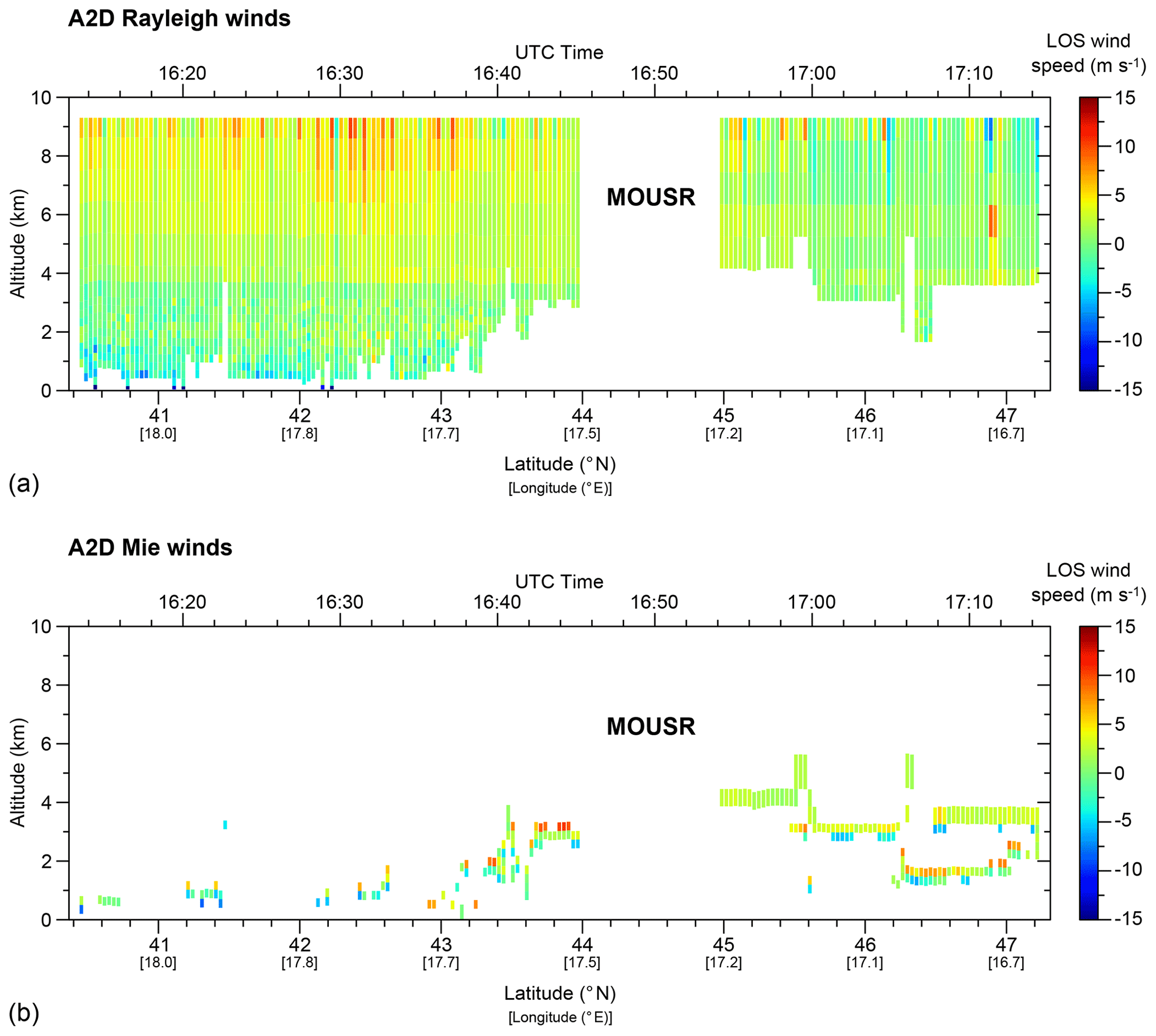
Figure 4LOS wind profiles (positive if winds are blowing away from the instrument) measured during the underflight on 22 November 2018 between 16:13 and 17:15 UTC along the Aeolus measurement track (white arrow in Fig. 2) using (a) the A2D Rayleigh and (b) Mie channels. White areas represent missing or invalid data due to low signal, e.g. below dense clouds. The data gap between 16:45 and 16:54 UTC is due to an interruption of the wind measurement during a different operation mode (MOUSR) of the A2D instrument that aimed at the detection of the Rayleigh background signals on the Mie channel.
Figure 4 shows the processed LOS Rayleigh and Mie winds plotted vs. latitude (and time) and altitude for the period of the Aeolus underflight on 22 November 2018. During the first section of the flight, cloud-free conditions led to nearly complete data coverage of the Rayleigh channel from the ground up to an altitude of 9 km. During the second half of the flight, dense mid-level clouds limited the extension of the Rayleigh wind profiles to above 4 to 5 km. The data gap in between is due to the MOUSR procedure mentioned above.
The range gate settings were identical for the Rayleigh and Mie channels and were chosen to sample the lowermost 3.5 km of the troposphere with the highest possible vertical resolution. Therefore, the integration time of the ACCD was set to 8.4 µs in the range gates from 7 to 10 (9.3 to 4.5 km), 4.2 µs in range gates 11 and 12 (4.5 to 3.5 km) and 2.1 µs in all of the remaining range gates towards the ground, corresponding to a height resolution of 1184, 592 and 296 m respectively. LOS wind speeds of up to 15 m s−1 were measured with the Rayleigh channel at altitudes between 8 and 9 km. Note that positive wind speeds are obtained when the A2D LOS unit vector points along the direction of the horizontal wind vector, i.e. the wind is blowing away from the instrument. This definition is in contrast to previous campaigns where winds blowing towards the instrument were defined as positive in accordance with a positive Doppler frequency shift. It was inverted in order to follow the sign convention of Aeolus, thereby allowing for the better comparison of different wind data sets. In the case shown here, northwesterly winds were present around the Adriatic Sea with horizontal wind speeds up to 50 m s−1 at an altitude of 9 km according to the ECMWF model. However, as the A2D was pointing towards the northeast along the Aeolus track, the projection of the horizontal wind vector onto the instrument's LOS was small, resulting in low measured wind speeds with a positive sign. At lower altitudes, the wind direction was the opposite, so that the wind was blowing towards the instrument, leading to slightly negative wind speeds.
In contrast to the Rayleigh channel, the Mie data coverage is rather poor due to the sparse cloud cover and low aerosol load during the flight. Wind data are mainly obtained from the cloud tops along the track. Due to the high optical density of the clouds, the laser was strongly attenuated, which prevented sufficient backscatter signal and valid Mie wind data over multiple range gates within and below the clouds. As a result, valid Mie wind data are often only obtained for one bin per profile or, if data from a subjacent range gate pass quality control, the wind data show a large systematic error. This is likely due to the skewness of the Mie fringe on the ACCD which influences the determination of the centroid position depending on the position of the cloud within the range gates. The same characteristics were observed for the other two Aeolus underflights; thus, the number of valid and good quality Mie wind data is very low compared with the Rayleigh channel. The scarce coverage of the Mie data and the high number of outliers due to the Mie fringe skewness in combination with the presence of thick clouds prevented a meaningful comparison with the Aeolus data that showed similarly poor Mie data coverage for the same reasons. Thus, further analysis of the A2D and Aeolus wind data is restricted to the Rayleigh channel.
3.3 Aeolus wind results from the underflight on 22 November 2018
When the Falcon aircraft was located at 42.8∘ N, 17.7∘ E at 16:34:56 UTC after about one-third of the common leg from Lecce to the Austrian–Hungarian border, Aeolus was just passing by, measuring winds in the same atmospheric volume along its path. A total of 66 s later, the satellite finished the common leg, while the Falcon arrived at the northern end of the track at 17:15 UTC, resulting in a maximum temporal distance between the wind data acquisitions of the airborne and satellite instruments of about 40 min. The wind data obtained with the Aeolus Rayleigh channel are depicted in Fig. 5. The profiles span the range from the ground to the lower stratosphere (21 km) with a vertical resolution of 0.25 km in the lowermost range gates up to an altitude of 2 km. In the altitude range between 2 and 13 km, the bin thickness is 1 km, whereas it is 2 km in the region above. Hence, a maximum of 15 range bins lie within the sampled altitude range of the A2D below 10 km. The selected range gate setting of Aeolus ensured accurate ground detection with the highest possible vertical resolution, which was crucial for determining potential wind biases during the commissioning phase of the mission. The data plotted in Fig. 5b are the wind speeds measured along the satellite's LOS which are denoted using an asterisk (LOS*) in the following in order to avoid confusion with the A2D LOS. Due to the larger off-nadir angle of relative to the normal direction at the measurement swath (considering the Earth curvature) compared with the A2D (20∘), the projection of the horizontal wind vector onto the satellite LOS* is generally larger and the measured wind speeds are therefore higher.

Figure 5(a) Aeolus observational geometry, and (b) Aeolus L2B LOS* Rayleigh winds (positive if winds are blowing away from the instrument) measured during the underflight on 22 November 2018 between 40.6 and 47.2∘ N. Only winds with an estimated wind error of less than 12 m s−1 are shown. Winds at altitudes above 10 km are outside of the measurement range of the A2D and are consequently greyed out. The figure was created based on a screenshot from the Aeolus data visualization tool, © VirES for Aeolus (https://aeolus.services/, last access: 25 November 2019).
The HLOS wind speed included in the L2B wind data product of Aeolus can be converted to the LOS* wind speed using the off-nadir angle ΘAeolus (see the Aeolus observational geometry in Fig. 5a):
The L2B product also contains the Rayleigh estimated wind error which is derived from the signal-to-noise level and the pressure and temperature sensitivity of the Rayleigh channel responses (Tan et al., 2017). Bins for which the estimated error is larger than 12 m s−1 are omitted in the diagram in Fig. 5. This leads to data gaps in the lower troposphere in the northern part of the common leg where dense low-level clouds strongly attenuated the laser beam and the backscattered signal from below the clouds, as also observed for the A2D. In accordance with the weather forecast, Aeolus measured strong winds in the southern part of the leg between 8 and 10 km, reaching LOS* wind speeds of up to 25 m s−1, whereas weaker winds were observed towards the north. Before comparing the A2D and Aeolus wind results from the selected underflight as well as from the entire campaign, the quality of the A2D data during WindVal III will be discussed in the following.
3.4 Assessment of the A2D performance by comparison with the 2 µm DWL
The accuracy and precision of the A2D Rayleigh wind results were evaluated by comparing them to the wind data obtained from the coherent 2 µm DWL, which was operated in parallel on the same aircraft and is characterized by a high accuracy of the horizontal wind speed of about 0.1 m s−1 and a precision of better than 1 m s−1 (Weissmann et al., 2005; Chouza et al., 2016; Witschas et al., 2017). For this purpose, the 3-D wind vectors measured with the 2 µm DWL were projected onto the A2D LOS axis. Moreover, the 2 µm measurement grid was adapted to that of the A2D by means of a weighted aerial interpolation algorithm, as introduced in Marksteiner et al. (2011). The latter was, in a similar fashion, also utilized for the comparison of the A2D and Aeolus data and will be described in the next section. By analogy with the results presented for selected flights of the WindVal II campaign in 2016 (Lux et al., 2018), a statistical comparison was performed that yielded the systematic and random error of the A2D Rayleigh winds for all underflights of the WindVal III campaign; the corresponding scatterplot and the results from the previous campaign, WindVal II, are depicted in Fig. 6a, while the respective statistical parameters are provided in Table 3.

Figure 6(a) Scatterplots comparing the A2D Rayleigh LOS winds with the 2 µm DWL winds for all Aeolus underflight legs from the WindVal III campaign in 2018 (green) and for all flights from the WindVal II campaign in 2016 (red). The corresponding probability density functions for the wind differences (A2D–2 µm), i.e. the A2D wind error, are shown in panels (b) and (c) for the two campaigns respectively. The solid lines represent Gaussian fits with the given centres and widths 2w.
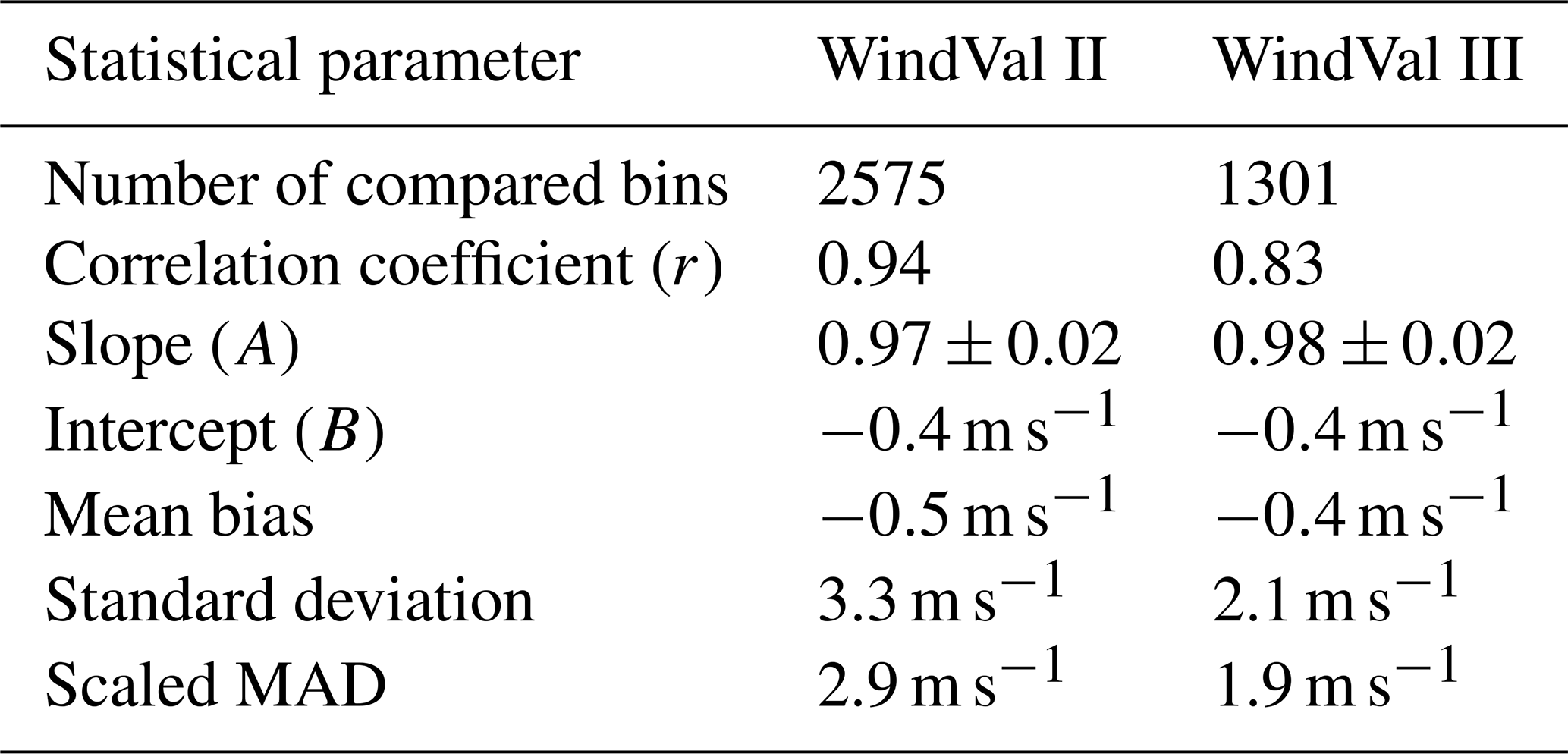
Table 3Results of the statistical comparison between the A2D Rayleigh channel and the 2 µm DWL wind data for all flights performed during the WindVal II campaign in 2016 and the WindVal III campaign in 2018. See the corresponding scatterplots in Fig. 6. The values are given as wind speeds measured along the A2D LOS. (MAD refers to median absolute deviation.)
In addition to the parameters provided in the insets of Fig. 6a, Table 3 also includes the slopes (A) and intercepts (B) of non-weighted linear fits applied to the two scatterplots. Here, vx and vy represent the wind speeds plotted on the abscissa and ordinate respectively. The standard error of the slope given in Table 3 was calculated according to
refers to the residuals of the linear regression.
During the WindVal II campaign, 12 research flights were performed with the primary focus of sampling high wind speeds and gradients related to the North Atlantic jet stream. Therefore, the number of wind results compared and the wind speed range are considerably larger than those of the WindVal III campaign, where generally weaker winds were encountered during the four satellite underflights in central Europe. Nevertheless, more than half as many A2D Rayleigh winds were included in the statistical comparison with the 2 µm DWL winds, as the WindVal III flights were preferentially conducted in cloud-free regions for the purpose of large data overlap with Aeolus. It should be noted here that the 2 µm DWL is very sensitive to weak backscatter return from clouds and aerosols due to its small-bandwidth coherent detection principle; thus, 2 µm DWL winds are even available for low scattering ratios (< 1.1), where insignificant Mie contamination of the A2D Rayleigh channel can be expected.
The WindVal III flight planning aimed to reduce the probability of heterogeneous cloud conditions which, in turn, increased the representativeness of the scan-retrieved volume winds obtained from the 2 µm DWL to the A2D LOS winds. Furthermore, the risk of large systematic errors in the Rayleigh channel, e.g. introduced by cirrus clouds affecting the transmit–receive co-alignment feedback loop, was minimized. Consequently, the scatterplot for WindVal III in Fig. 6a features fewer outliers than that of WindVal II. The more homogeneous atmospheric conditions and the implementation of the fibre scrambler to diminish the internal reference frequency noise result in a significant reduction in the random error (by more than 30 % to less than 2 m s−1), while the mean bias of −0.4 m s−1 is comparable to the previous campaign (−0.5 m s−1).
In addition to the standard deviation, the median absolute deviation (MAD) was determined to quantify the random error of the A2D wind speed measurements. It is defined as the median of the absolute variations of the measured wind speeds from the median of the wind speed differences:
Compared with the standard deviation, the MAD is more resilient to outliers and, thus, a more robust measure of the variability of the measured wind speeds. When the random wind error is normally distributed, the MAD value, multiplied by 1.4826 (scaled MAD), is identical to the standard deviation. The larger number of outliers in the scatterplot for the WindVal II campaign manifests in a larger discrepancy between the standard deviation (3.3 m s−1) and the scaled MAD value (2.9 m s1) compared with WindVal III (2.1, 1.9 m s−1). The random error can also be approximated from probability density functions (PDFs), illustrating the frequency distribution of the wind speed differences vA2D–v2 µm, i.e. the wind error (Fig. 6b, c). Since the wind error does not follow a perfect Gaussian distribution for both campaigns, there is a deviation between the mean bias values and the centre of the Gaussian fits. For the same reason, the width of the fits is narrower than twice the standard deviations which also consider the outliers.
For adequate comparison of the A2D wind profiles with the Aeolus wind data, two major aspects have to be considered. First, the different horizontal and vertical resolutions of the two instruments necessitate an adaptation of the A2D measurement grid to that of Aeolus. Second, the different viewing geometries of the wind lidars need to be taken into account. Since both instruments measure only one component of the horizontal wind vector along their respective LOS, information on the wind direction is required in order to determine the wind speed difference of the A2D and Aeolus resulting from the different LOS directions.
4.1 Adaptation of the measurement grid
Due to the fact that the horizontal resolution of Aeolus is much coarser than that of the A2D (see Table 1), interpolation of the A2D wind measurements onto the Aeolus measurement grid is required. In the framework of previous A2D campaigns, an aerial weighted averaging algorithm (Marksteiner et al., 2011; Marksteiner, 2013) was developed to compare the A2D wind results with the data obtained from the 2 µm reference wind lidar (Lux et al., 2018). The grid adaptation procedure used in this study is based on that algorithm. Each valid A2D range bin covering an Aeolus range bin is allocated both horizontal and vertical weights depending on the size of its contribution to the total area of the Aeolus bin, as illustrated in Fig. 7.
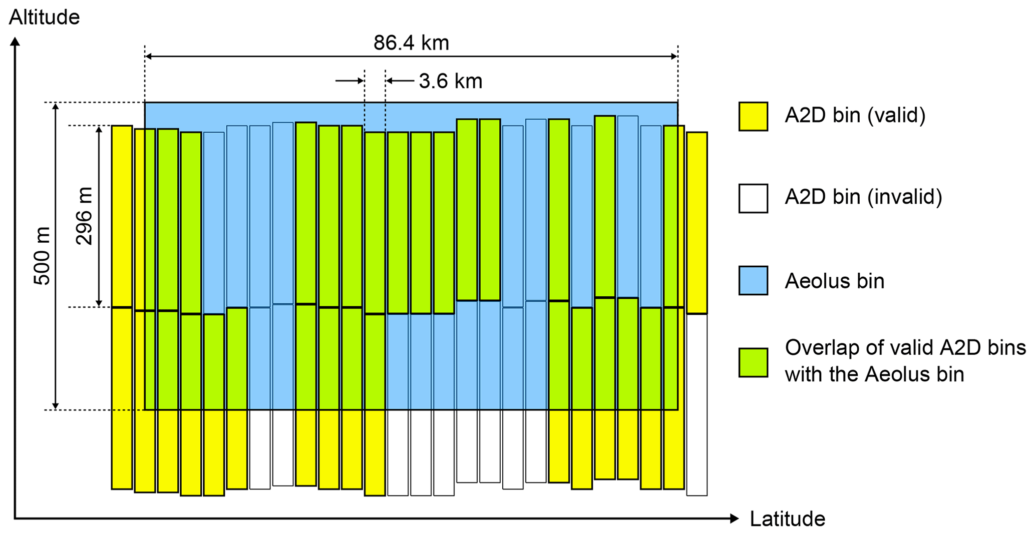
Figure 7Schematic illustrating the different horizontal and vertical resolutions of Aeolus (blue bin) and the A2D (yellow bins) for typical range gate settings (Aeolus: 500 m vertical resolution; A2D: 296 m vertical resolution). White bins indicate invalid A2D observations, while the green area represents the overlap of valid A2D bins with the Aeolus bin. For the aerial weighted averaging algorithm, the contributions of each valid A2D wind value to the wind value allocated to the composite bin are weighted by the overlap of the respective A2D bins with the Aeolus bin considered. The ratio of the green to the blue area is defined as the coverage ratio and is used as a quality control parameter (see Sect. 4.5).
Hence, for each Aeolus range bin a weighted average from the A2D contributions can be calculated. Moreover, the coverage ratio that determines the coverage of an Aeolus range bin by valid A2D bins is calculated as a measure of the representativeness of A2D winds within an Aeolus range bin. Especially in regions with strong wind shear within the area of an Aeolus range bin as well as sparse coverage, large representativeness errors are possible, e.g. when the A2D bins only cover the area of an Aeolus bin where high wind speeds reside, while lower wind speeds within the Aeolus bin are not covered. The influence of the coverage ratio on the statistics of the wind comparisons is discussed in Sect. 4.5. Additionally, the mean distance of the horizontal centres of the A2D bins covering an Aeolus bin to the latter's bin centre was defined as a second adjustable parameter that potentially influences the outcome of the statistical comparison.
4.2 Consideration of the different viewing geometries
A visual comparison of the A2D Rayleigh winds in Fig. 4a, measured during the underflight on 22 November 2018, with the corresponding Aeolus L2B Rayleigh wind curtain shown in Fig. 5 reveals large discrepancies. This is due to the fact that the viewing angles of the two instruments differ from each other. First of all, the off-nadir angles are different, as stated above (, ). Additionally, depending on the wind speed and direction along the flight track, the heading angle of the aircraft deviates from the true (course correction angle due to crosswind), resulting in a varying azimuth angle of the A2D. The situation is illustrated in Fig. 8, which shows the flight track of the aircraft along the satellite measurement swath and the respective horizontal viewing directions of the A2D and Aeolus at a selected position on the track. While the azimuth angle of the A2D was around 68∘, it was 80∘ for Aeolus. As a result, the two instruments measured different components of the horizontal wind vector projected onto the respective LOS vectors. In order to convert the A2D LOS winds to A2D LOS* winds, i.e. A2D winds that would have been measured if it was pointing in the same direction as the satellite instrument, both the off-nadir and the azimuth angle need to be considered. In a first step, the A2D LOS winds are converted to A2D HLOS winds by analogy with Eq. (1). Then, the real wind speed difference Δ that results from the different azimuth angles of the two instruments has to be determined and added to the actual wind speed measured by the A2D:
The determination of Δ requires an additional source of information. Therefore, model wind data from the ECMWF, which are included in the Aeolus L2C data product, were utilized. Knowledge of the zonal (u) and meridional (v) wind components allows for the calculation of the wind speed difference introduced by the different azimuth angles of the A2D (φA2D) and Aeolus (φAeolus) as follows:
Using the above-mentioned azimuth angles for the two instruments ( and ), the wind speed difference Δ can be larger than 5 m s−1 for typical zonal and meridional wind speeds of ±30 m s−1, as shown in the inset of Fig. 8. Only when the horizontal wind vector bisects the angle between the A2D and the Aeolus azimuth angle, which is for a wind direction of ( in the present example, does the wind speed difference vanish (Δ=0). On the contrary, the deviation reaches a maximum when the horizontal wind vector is perpendicular to the previously mentioned case (−16 or 164∘).
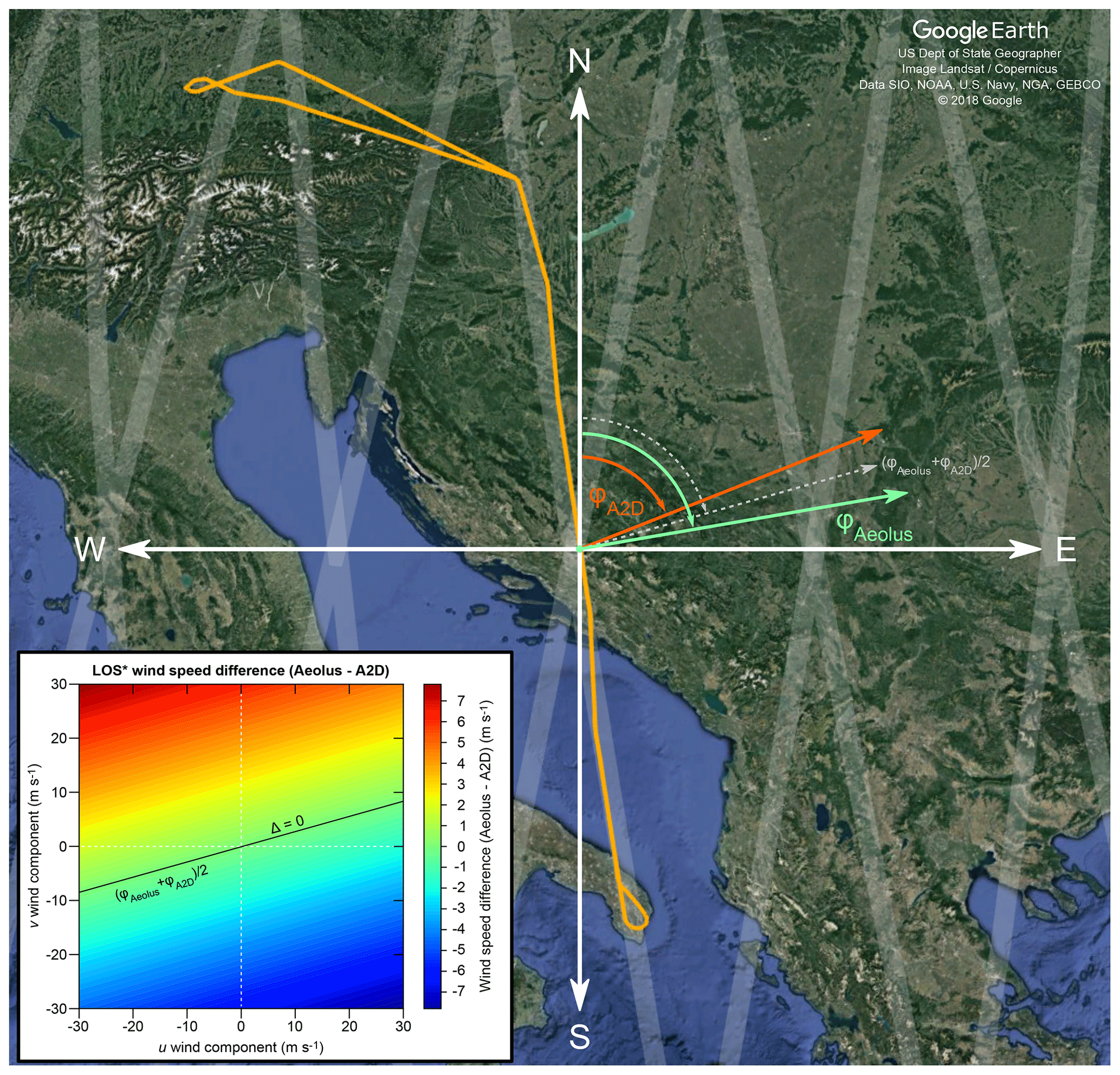
Figure 8Diagram illustrating the different azimuth angles of Aeolus (green arrow) and the A2D (orange arrow), using the underflight on 22 November 2018 (indicated by the orange flight track) as an example (background image: © 2018 Google). The inset depicts the dependence of the LOS* wind speed difference on the zonal (u) and meridional (v) wind components for azimuth angles of φA2D=68 and . When the azimuth angle of the wind vector meets the condition , i.e. the wind direction is 74∘ (dashed grey arrow), the LOS* wind speed difference Δ is zero.
As the Aeolus azimuth angle is generally around 80∘ at midlatitudes on ascending orbits, and the A2D azimuth angle is around 68∘ when flying on ascending satellite tracks, the plot is representative for all underflights of the WindVal III campaign. Thus, it can generally be stated that the meridional wind component predominantly influences the wind speed difference Δ. In summary, one could conclude that the azimuth correction is essential for the accurate comparison of the A2D and Aeolus winds.
Despite the high accuracy and precision of the 2 µm DWL, the model data were utilized for the azimuth correction due to their full coverage. In contrast, the coherent detection 2 µm DWL data exhibit gaps in clear air regions, preventing the correction of many wind results obtained with the A2D Rayleigh channel. It should be mentioned that, in principle, the adapted A2D wind results can potentially be impacted by model error (Schäfler et al., 2020). However, the comparison of the ECMWF model winds, averaged onto the Aeolus grid, with the 2 µm DWL wind data showed excellent agreement (a bias below 0.1 m s−1 and a random error ≈2 m s−1) without any significant outliers over the entire campaign (Witschas et al., 2020). Moreover, for typical azimuth angles of the two instruments, as mentioned above, the maximum error of the correction term Δ resulting from a potential model error of 1 m s−1 for both the u and v components or a potential model error of the wind direction of 3∘ accounts for less than 0.2 m s−1, which is acceptable given the A2D random error of about 2 m s−1.
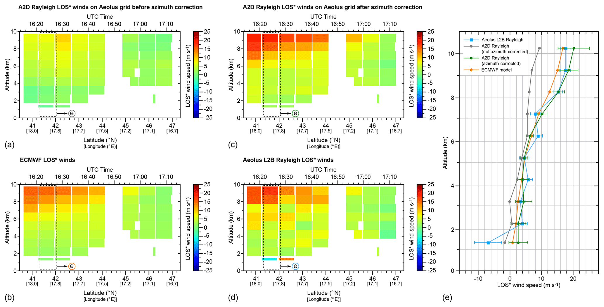
Figure 9LOS* wind profiles obtained during the underflight on 22 November 2018 between 40.5 and 47.2∘ N: (a) A2D Rayleigh winds averaged onto the Aeolus measurement grid for an off-nadir angle of 37∘ without azimuth correction, (b) ECMWF model winds, (c) A2D Rayleigh winds with azimuth correction and (d) Aeolus L2B Rayleigh winds. White areas represent missing or invalid data for one of the two instruments, e.g. below dense clouds. Only Aeolus Rayleigh LOS* winds with an estimated error below 4.8 m s−1 were considered valid. The wind profile for one selected Aeolus observation is shown in panel (e) along with the corresponding profiles of the other three data sets. The error bar for the Aeolus winds (blue squares) represents the estimated error included in the L2B product, whereas the error bar for the azimuth-corrected A2D winds (green dots) corresponds to the weighted standard deviation of all A2D bins contributing to the respective Aeolus bin. For the uncorrected A2D winds (grey dots), the error bars were omitted for the sake of clarity.
Finally, the azimuth-corrected A2D HLOS, i.e. the A2D HLOS*, wind speeds are multiplied by the factor (see Eq. 1) to obtain the A2D LOS* winds. The resulting wind curtains are depicted in Fig. 9.
Figure 9a shows the A2D Rayleigh winds averaged onto the Aeolus measurement grid for an off-nadir angle of 37∘ without azimuth correction, and Fig. 9b shows the Aeolus L2C Rayleigh winds, i.e. LOS* winds based on ECMWF model data (from the Aeolus L2C product). The A2D Rayleigh winds after azimuth correction (A2D LOS* winds) are shown in Fig. 9c, and the Aeolus L2B Rayleigh winds are depicted in Fig. 9d. Moreover, the wind profile for one selected Aeolus observation and the corresponding profiles of the other three data sets are shown in Fig. 9e. Here, the error bar for the Aeolus winds (blue squares) represents the estimated error included in the L2B product, while the error bar for the azimuth-corrected A2D winds (green dots) corresponds to the weighted standard deviation of the A2D winds from those bins that overlap with the respective Aeolus bin. Only Aeolus LOS* winds with an estimated error below 4.8 m s−1 (HLOS of 8 m s−1) were considered valid. A comparison of the curtain plots and the selected wind profiles demonstrates the necessity of the azimuth correction. Due to the strong meridional wind especially in the upper range gates of the A2D at the beginning of the common leg, large wind speed differences (Δ > 5 m s−1) were present between Aeolus and the uncorrected A2D data (grey dots); these differences were compensated for by the azimuth correction as explained above. Hence, the adapted A2D Rayleigh winds show much better agreement with both the Aeolus Rayleigh winds and the model data. The weighted standard deviation of the A2D winds, indicated by the error bars, represents a measure of the variability of the A2D winds within the compared Aeolus bin. The values are of the order of 2 to 4 m s−1 and are determined by both the random error of the A2D and the horizontal and vertical wind gradients within the respective Aeolus bin.
4.3 Statistical comparison of A2D and Aeolus with ECMWF data
The adaptation of the A2D data to the Aeolus measurement grid and LOS viewing direction allowed for a statistical comparison of the measured LOS* wind speeds with each other as well as with model wind data from the ECMWF. The latter will be presented in this section, while the lidar–lidar comparison is subject of the next section. Note that the error of the LOS* wind speed is the actual instrument error of Aeolus, which is also the reason why this parameter, and not the HLOS* wind included in the product, was chosen for the wind comparison. The scatterplot in Fig. 10a shows the correlation of the A2D Rayleigh winds with the ECMWF model data for the underflight on 22 November 2018. The scatter points are colour-coded with respect to the bottom altitude of the bin used for comparison. The plot shows good correspondence of the A2D winds with the model data for altitudes below 7 km, but it also reveals a positive mean bias of the A2D winds of 1.4 m s−1 which is evident over the entire wind speed range. Wind speed differences above 2 m s−1 are especially present at higher altitudes (light brown scatters). As the accuracy of the model data is assumed to be better than that of the A2D, with a nearly vanishing bias and low random error around 2 m s−1 (Witschas et al., 2017, 2020), it is used as the reference. The bias of the A2D winds is most likely related to the incomplete telescope overlap close to the aircraft resulting in a reduced backscatter signal as well as a systematic wind error (Paffrath et al., 2009). For the scatterplot shown in Fig. 10a, the scaled MAD of 1.6 m s−1 is significantly larger than the standard deviation (1.4 m s−1), indicating that the wind speed differences are not normally distributed, which is primarily owing to the positively biased winds measured at higher altitudes.
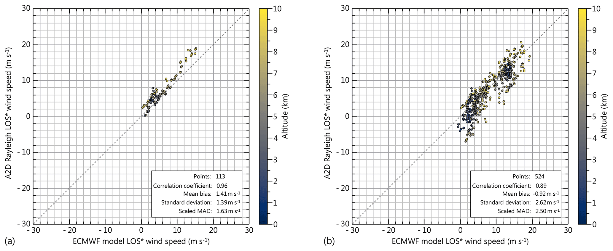
Figure 10Scatterplots comparing the A2D Rayleigh LOS* winds with the ECMWF model LOS* winds (a) for the wind scene on 22 November 2018 between 16:13 and 17:15 UTC and (b) for all underflights of the WindVal III campaign. The data points are colour-coded with respect to the bottom altitude of the respective bins used for comparison.
By analogy with the flight leg discussed above, the other co-located wind observations of the campaign listed in Table 2 were analysed.
The statistical values derived from the comparison of the different data sets are summarized in Table 4. Table 4 also includes the parameters from the A2D–2 µm comparison discussed in Sect. 3.4 after the conversion to LOS* wind speeds. For the results from the comparison of the 2 µm DWL data with Aeolus, please refer to Witschas et al. (2020). When comparing the A2D to the model data from all Aeolus underflights (Fig. 10b), a mean bias of −0.9 m s−1 is calculated, which is in fair agreement with the bias determined from the 2 µm reference lidar (−0.7 m s−1 LOS*, corresponding to −0.4 m s−1 LOS) considering the smaller data coverage of the 2 µm DWL compared with the model. The intercept of the linear regression function is even below −1 m s−1, while the slope deviates from the ideal case (A=1) by 3 %. This slope error is most likely related to an imperfect calibration of the Rayleigh channel. In particular, differences in atmospheric pressure and temperature encountered during the calibration procedure and the wind scene give rise to a mismatch between the derived calibration parameters and the actual Rayleigh channel behaviour during the underflight (Zhai et al., 2020). The scatterplot also shows that most of the over- and underestimated A2D winds are measured either at high altitudes (> 8 km) or very close to the ground (< 2 km). While the deviations close to the aircraft can be explained by the incomplete telescope overlap, the larger wind speed differences at lower altitudes are probably related to the influence of aerosols in the planetary boundary layer that cause Mie contamination of the Rayleigh signal and, in turn, introduce systematic errors of the winds measured in this region. Note that, in contrast to the A2D, a so-called cross-talk correction is performed for the satellite instrument to minimize such errors. Despite these error sources, the standard deviation of 2.6 m s−1 and scaled MAD of 2.5 m s−1 of the A2D Rayleigh winds are considerably lower than values observed during previous airborne campaigns, as discussed above. The fact that the random error is even lower than the (LOS*-converted) values obtained from the 2 µm DWL comparison (3.4 m s−1) can be explained by the coarser horizontal and vertical resolution of the model winds included in the L2C product, which is provided on the same grid as the L2B product. Consequently, the number of A2D wind results that are averaged onto the model grid is larger than for the finer 2 µm grid (by a factor of ≈2.5), thereby reducing the variability in the bin-to-bin wind comparison (by a factor of ).
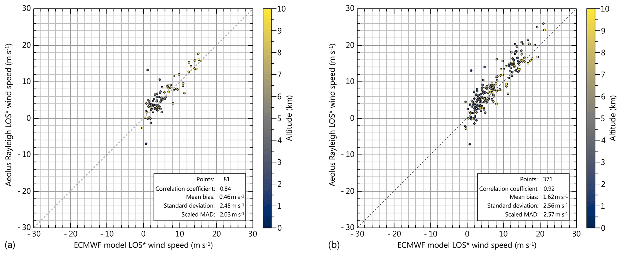
Figure 11Scatterplots comparing the Aeolus L2B Rayleigh LOS* winds with the ECMWF model LOS* winds (a) for the wind scene on 22 November 2018 between 16:13 and 17:15 UTC and (b) for all of the underflights from the WindVal III campaign. The data points are colour-coded with respect to the bottom altitude of the respective bins used for comparison.
Figure 11 depicts the statistical comparison of the Aeolus Rayleigh winds with the ECMWF model data. Here, a positive mean bias of 0.5 m s−1 is determined for the wind scene on 22 November 2018, while the random error is larger (a standard deviation of 2.5 m s−1, and a scaled MAD of 2.0 m s−1) than for the A2D winds for that scene. This is mainly due to the two outliers that also become apparent in the Aeolus wind curtain (Fig. 9d) at an altitude of about 1.5 km. Here, the small bin size of 250 m entails a poor signal-to-noise level, resulting in a large random wind error that is close to the estimated error threshold of 4.8 m s−1 applied to the curtains in Fig. 9. Comparing the Aeolus LOS* winds with the model data for the entire campaign (Fig. 11b), a mean bias of 1.6 m s−1 and a random error of 2.6 m s−1 (scaled MAD) are derived.
Figure 12Scatterplots comparing the Aeolus L2B Rayleigh LOS* winds with the A2D Rayleigh LOS* winds (a) for the wind scene on 22 November 2018 between 16:13 and 17:15 UTC and (b) for all of the underflights from the WindVal III campaign. The data points are colour-coded with respect to the bottom altitude of the respective bins used for comparison.
Table 4Results of the statistical comparison between the A2D Rayleigh, the Aeolus Rayleigh and the ECMWF LOS* wind speeds for all of the underflights performed during the WindVal III campaign. See the corresponding scatterplots in Fig. 11 (that refer to the last three columns in this table). The first column includes the data from Table 3 after the conversion of the wind speeds to the satellite's LOS* (37∘ off-nadir angle). Please note that different horizontal and vertical averaging lengths apply to the different comparisons (see text for details).
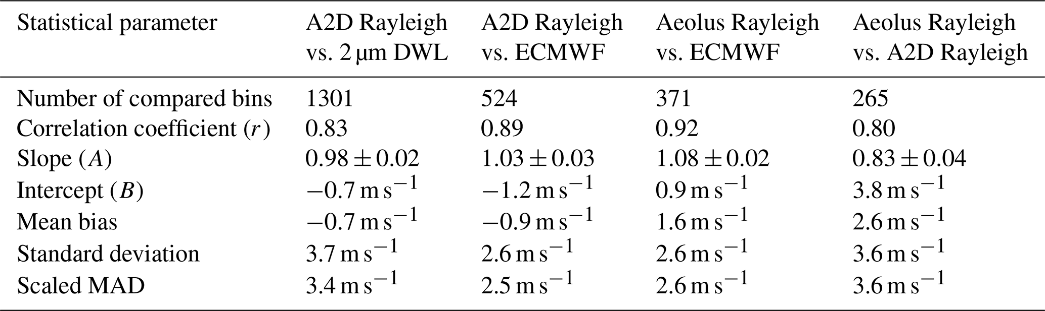
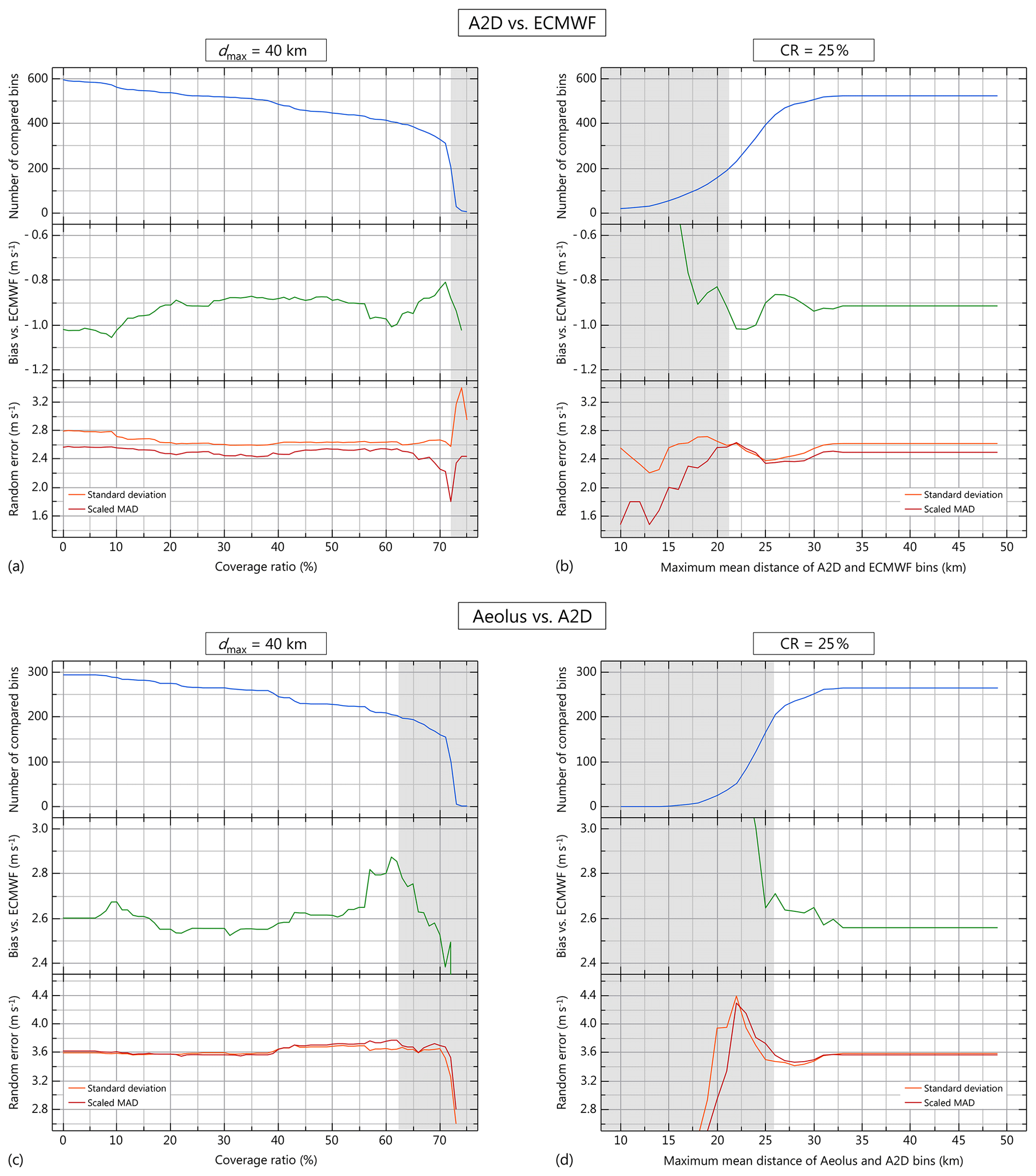
Figure 13Influence of the (a, c) coverage ratio and (b, d) horizontal distance threshold on the statistical parameters resulting from the A2D–ECMWF comparison (a, b) and the Aeolus–A2D comparison (c, d). The top panels of each subfigure depict the number of bins included in the statistical comparison, the middle panels show the bias and the bottom panels illustrate the random error (standard deviation and scaled MAD) depending on the respective threshold parameter. Results for which the number of compared bins is below 200 are considered statistically insignificant and are indicated as grey shaded areas.
4.4 Statistical comparison of A2D and Aeolus data
The scatterplots comparing the Aeolus and A2D Rayleigh winds are depicted in Fig. 12. For the underflight on 22 November 2018, a negative bias of around −0.8 m s−1 for the Aeolus winds with respect to the A2D data is apparent (Fig. 12a). The small discrepancy between this value and the respective biases to the ECMWF model discussed in the previous section (0.5–1.4 m s m s−1) can be explained by the dissimilar wind data coverage of the airborne and satellite instruments. The latter also results in different numbers of scatter points for the comparisons of the three data sets with one another. It should be noted that the statistical results from the mutual comparisons only slightly deviate from the values shown (by less than 0.2 m s−1) when restricting the respective data sets to those bins where both instruments have valid wind data. The large spread in the Aeolus wind data compared with the A2D winds in Fig. 12a results from the fact that the random errors of the two lidar instruments with respect to the model winds approximately add up quadratically according to
This leads to a standard deviation of 3.0 m s−1 and a slightly smaller scaled MAD of 2.9 m s−1. Even larger variances are observed when comparing the data from all of the underflights (Fig. 12b), where both the standard deviation and the scaled MAD are around 3.6 m s−1. The actual systematic and random error of Aeolus can be estimated from the Aeolus–A2D comparison when the A2D accuracy and precision are taken into account. Following this approach, the observed bias of 2.6 m s−1 translates to an actual bias of 2.6–0.7 m s m s−1 or 2.6–0.9 m s m s−1 when considering the negative bias of the A2D Rayleigh channel with respect to the 2 µm DWL and the model respectively. Using Eq. (6), the random error of the Aeolus winds is approximated to be [(3.6 m s−1)2–(2.6 m s−1)2] m s−1. Hence, the A2D and Aeolus Rayleigh channels show a very similar precision of about 2.5 m s−1, although the underlying reason for the Aeolus random error is of a different nature, as explained below. The derived Aeolus Rayleigh accuracy and precision are in fair agreement with the results from the Aeolus–2 µm comparison described in Witschas et al. (2020) where a positive bias of 2.1 m s−1 (HLOS) and scaled MAD of 4.0 m s−1 (HLOS) were determined, corresponding to LOS* values of 1.3 and 2.4 m s−1 respectively. A positive bias of the L2B Rayleigh winds (1.5 m s−1 HLOS) was also verified by comparative measurements using a ground-based wind lidar located in southern France in January 2019 (Khaykin et al., 2020).
For the campaign time and region, the bias of the L2B Rayleigh winds is beyond the mission requirements of Aeolus which should provide an accuracy of 0.7 m s−1 in HLOS winds (0.4 m s−1 LOS*) on a global scale, while the HLOS random error is required to be below 1 m s−1 (0.6 m s−1 LOS*) in the planetary boundary layer, 2.5 m s−1 (1.5 m s−1 LOS*) in the troposphere and 3 to 5 m s−1 (1.8 to 3.0 m s−1 LOS*) in the stratosphere in order to ensure a positive impact on the weather forecast by assimilating the wind data in numerical weather prediction models (ESA, 2016). The wind bias is owed to the fact that the mission was still in the commissioning phase at the time of the campaign. In this period, instrumental drifts were observed to result in a long-term change in the incidence angle on the Rayleigh spectrometer and, thus, systematic Rayleigh wind errors. Moreover, the emitted energy of the laser of 60 mJ was below the target value of 80 mJ which, combined with presumed losses in the receive path, led to significantly lower signal-to-noise levels (by about a factor of 2.5 to 3) than expected (Reitebuch et al., 2019). As a consequence, the random error did not meet the system requirements for the troposphere in the early phase of the mission. Considerable improvement of the accuracy and precision of the Aeolus data is expected after correction for instrumental drifts and after increasing the laser output energy via system adjustments respectively.
In conclusion, due to the preliminary nature of the Aeolus L2B wind product, the Rayleigh winds exhibit relatively large systematic and random errors that are higher than the mission requirements (ESA, 2016). However, it should also be stated that the representativeness of the statistical results shown here is limited by the relatively small data set obtained from the WindVal III validation campaign. A strategy for increasing the number of winds compared and, hence, the representativeness of the Aeolus Cal/Val results in forthcoming campaigns is described in Sect. 4.6.
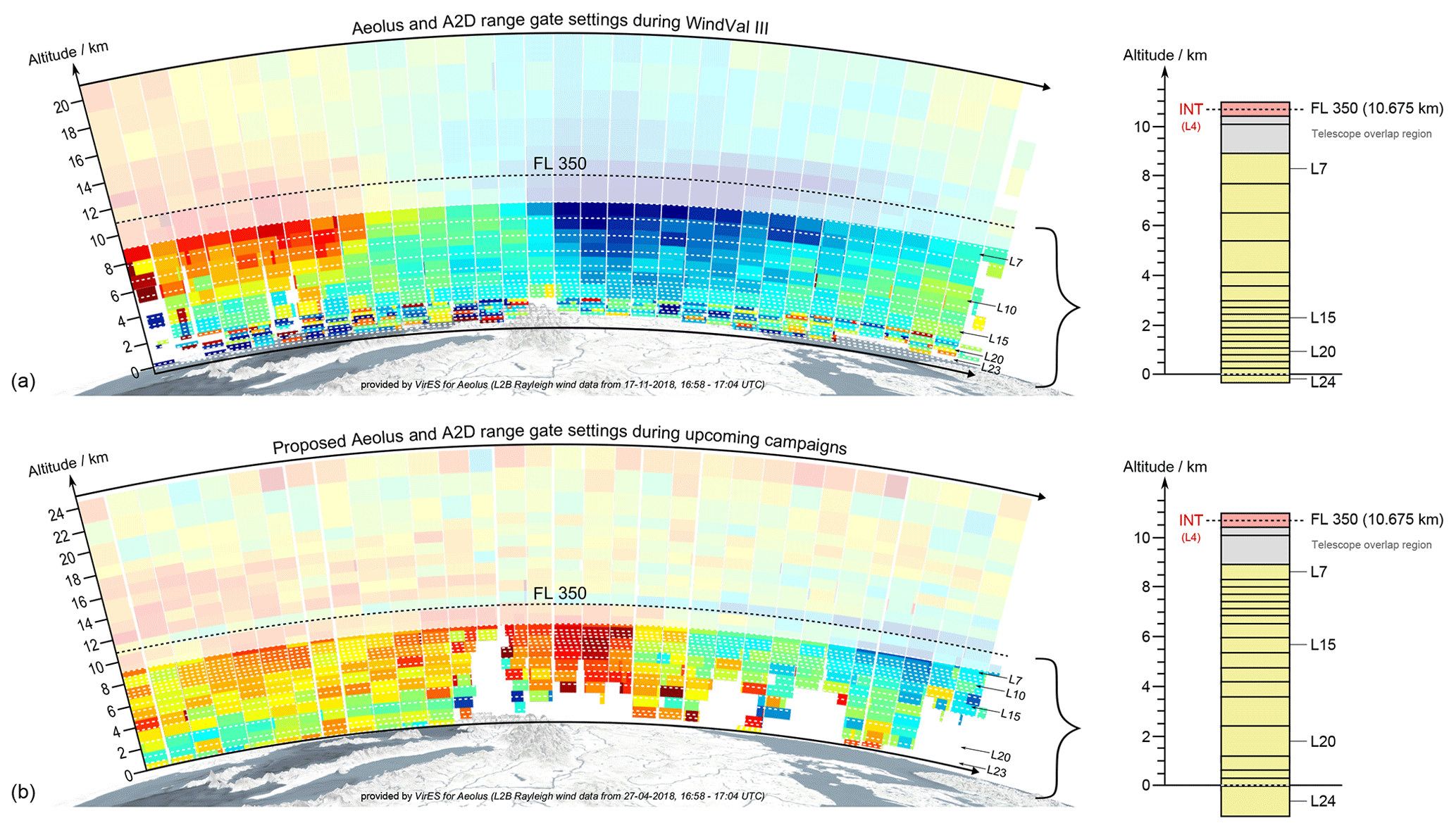
Figure 14Diagram illustrating (a) the A2D range gate setting used during the WindVal III campaign and (b) an optimized range gate setting planned to be used in forthcoming airborne validation campaigns. The left part of the figure shows exemplary Aeolus L2B Rayleigh wind curtains with indicated bin altitudes of the A2D range gates (white dashed lines) assuming a flight altitude of about 10675 m (FL 350). The corresponding vertical range gates (atmospheric layers; L) are also depicted on the right. Due to the incomplete telescope overlap, the wind data from the first 1.5 km below the aircraft show increased wind errors and are consequently not used. The figure was created based on screenshots from the Aeolus data visualization tool, © VirES for Aeolus (https://aeolus.services/, last access: 12 November 2019).
4.5 Influence of the coverage ratio and mean distance thresholds
The aerial weighted averaging algorithm described in Sect. 4.1 runs the risk of large discrepancies between the averaged A2D wind and the compared Aeolus L2B or ECMWF model wind from the L2C product if the measurement bin from the respective Aeolus data product is only sparsely covered by A2D bins, especially in regions with strong wind shear. An additional potential representativeness error may arise from overly large spatial separation between the A2D bins covering an Aeolus bin and the bin centre of the latter. Therefore, two tunable threshold parameters were defined for the statistical comparisons described in the previous section. While the minimum overlap of the compared bins (coverage ratio threshold, CR) was set at 25 %, the upper threshold of the mean distance dmax between the Aeolus bin centre and the bin centres of all overlapping A2D bins was set at 40 km. The influence of the two parameters on the statistical parameters retrieved from the A2D–ECMWF comparison and the Aeolus–A2D comparison is shown in Fig. 13. Figure 13 a and c illustrate that the choice of the coverage ratio has no significant effect on the bias and random error (< 0.2 m s−1) for values below 50 %. At higher thresholds, the number of compared winds becomes considerably lower, resulting in a stronger dependence of the statistical values on the coverage ratio. Therefore, the results of the respective wind comparisons for which the number of compared bins is below 200 are considered statistically insignificant and are indicated using grey shaded areas in Fig. 13.
Regarding the maximum mean distance between the Aeolus L2B/L2C bin and the covering A2D bins (see Fig. 12a and c), a strong impact is observed for dmax < 30 km, as the number of winds compared is drastically reduced. Given the horizontal length of the Aeolus bin of about 86 km, the statistical parameters remain constant for distances from the bin centre above ≈40 km. Based on the above-mentioned considerations, relaxed threshold parameters of CR =25 % and dmax=40 km were found to provide an optimal trade-off between comparability and an acceptable number of representative composite A2D bins used for comparison. In this respect, the second threshold parameter dmax was effectively switched off to maximize the number of data points. However, the adaptation of the two parameters is advisable for wind scenes exhibiting more heterogeneous atmospheric conditions, as these are more prone to large representativeness errors if A2D data coverage is sparse. The same holds true for the comparison of Mie winds, which is envisaged for future campaigns.
4.6 Optimization of A2D range gate settings
It should be noted that only a relatively small number of bins are compared, especially for the Aeolus–A2D comparison (265). This is primarily due to the vertical sampling settings of the A2D and Aeolus that was used which had many small range gates in the lower troposphere (Fig. 14a), where Aeolus winds often exhibit large estimated wind errors above the threshold useable for comparison. The overlap of valid wind data from the two instruments was therefore limited to the range between 2 and 9 km where the vertical resolution of both wind lidars was set to be coarser. With a view to the upcoming campaigns during the operational phase of the Aeolus mission, an extended statistical comparison and, hence, more detailed validation can be accomplished by adapting the vertical sampling strategy such that a higher number of small and medium-sized range gates are located at altitudes between 4 and 8 km at the expense of lower resolution towards the ground. A proposed optimized A2D range gate setting is illustrated in Fig. 14b, depicting exemplary Aeolus Rayleigh wind curtains from November 2018 and April 2019 with overlaid bin borders of the A2D (dashed lines) for an aircraft flight altitude of 10675 m (35 000 feet, flight level 350). The diagram shows that the Aeolus range gate settings were already modified after the end of the commissioning phase in January 2019, providing higher resolution in the upper troposphere. By using range gates with 296 and 592 m thickness for the A2D in the same region, the number of bins compared can be significantly increased. Furthermore, vertical sampling with higher resolution at altitudes close to the tropopause allows for the resolution of jet streams that often reside in this region, thereby delivering wind data over a wider wind speed range that can be included in the statistical comparison. This will additionally improve the significance of the statistical comparison, as the error in the fit parameters derived from the linear regression will be reduced according to Eq. (2a). The tropopause region is of particular interest, as increased ECMWF model errors with respect to the 2 µm DWL have been observed in recent studies (Schäfler et al., 2020).
In addition to the validation of the L2B wind speeds, the comparative analysis of the A2D and Aeolus wind results from forthcoming airborne campaigns will rather be dedicated to case studies of special scenes. In this context, it is anticipated that the different data coverage of the respective Rayleigh and Mie channels will be investigated under various atmospheric conditions. Moreover, future studies will focus on the origin of large outliers in the L2B wind product that show a low estimated error but large deviations from the airborne measurements. Here, the quality control mechanisms that have been developed and refined for the A2D over the past few years can potentially be used to optimize the L2B processor algorithms.
The airborne wind validation campaign WindVal III was carried out in central Europe only 3 months after the launch of ESA's Earth Explorer mission Aeolus in August 2018. More than 3000 km of the Aeolus measurement swath was covered during four underflights with the DLR Falcon aircraft carrying the airborne prototype of the Aeolus payload as well as a coherent Doppler wind lidar. A2D data are available from three underflights and comprise more than 11 h of wind measurements to be compared with the satellite data. Due to the sparse data coverage of the A2D and Aeolus Mie channels, which was accepted in the flight planning for the benefit of better coverage of the respective Rayleigh channels, only the latter were investigated further in this study.
The WindVal III campaign has provided several lessons that will be considered in the forthcoming Cal/Val campaigns. Above all, it is anticipated that dedicated flights with higher aerosol loading and larger cloud cover will be conducted to allow for an assessment of the Mie channel performance. In particular, wind measurements in thin cirrus clouds are expected to yield valid Mie data over multiple range bins across the wind profile, as observed during flights in the North Atlantic region in the framework of the NAWDEX campaign in 2016 (Lux et al., 2018). Proper comparison of the A2D and Aeolus wind results required the adequate averaging and consideration of the different viewing geometries. An aerial interpolation algorithm was used for the adaptation of the A2D data to the Aeolus measurement grid, whereas conversion of the measured A2D LOS winds to the satellite LOS was realized with the aid of model wind data. This procedure is not only of relevance for future validation campaigns employing the A2D but also for other wind lidars that do not have the capability to retrieve the entire wind vector. The harmonized data sets were then compared to each other as well as to ECMWF model wind data, which was used as a reference. Two tunable threshold parameters were introduced to the algorithm, and their influence on the correlation of the data sets was studied. The statistical comparison revealed biases of −0.9 and +1.6 m s−1 for the A2D and Aeolus LOS* Rayleigh wind speeds with respect to the ECMWF model respectively. Intercomparison of the two wind lidars showed a positive bias of the Aeolus Rayleigh LOS* winds with respect to the A2D of 2.6 m s−1, while the spread between the two data sets of 3.6 m s−1 resulted from the respective random errors that added up quadratically. Considering the systematic and random error of the A2D, the accuracy and precision of the Aeolus Rayleigh LOS* winds are determined to be +1.7 and 2.5 m s−1, which is in line with the results from other validation studies performed for the commissioning phase of the Aeolus mission (Khaykin et al., 2020; Witschas et al., 2020).
The accuracy and precision of the A2D winds were significantly better than in previous campaigns, whereas the Aeolus performance did not meet the formulated requirements of the mission for the studied wind scenes that took place during its commissioning phase. However, improvement of the satellite data quality is expected due to a refinement of the Aeolus processor, considering instrumental drift, and due to an enhancement of the laser output power. For future airborne validation campaigns, an optimized range gate setting of the A2D will be implemented to increase the overlap with valid Aeolus wind data from the two instruments as well as to ensure better sampling of strong wind gradients and higher wind speeds in the upper troposphere. Furthermore, a larger number of underflights will be performed to increase the validity of the wind data comparison. This will also allow for various case studies that aim to optimize the Aeolus processor algorithms.
The work in this paper includes preliminary data (not fully calibrated/validated and not yet publicly released) from the Aeolus mission, which are part of the European Space Agency (ESA) Earth Explorer Programme. Further data quality improvements, including, in particular, a significant product bias reduction, will be achieved before the public data release. This analysis was performed in the framework of the Aeolus Scientific Calibration and Validation Team (ACVT). The A2D and 2 µm DWL data used in this paper can be provided upon request to Christian Lemmerz (Christian.Lemmerz@dlr.de). Aeolus data were obtained from the VirES visualization tool, VirES for Aeolus: https://aeolus.services/ (last access: 12 November 2019).
OL and CL conducted the A2D wind observations. CL was the PI of the WindVal III campaign. OL, FW and UM analysed the A2D data and developed the methodology to compare the data sets. BW conducted the 2 µm DWL measurements. SR processed the 2 µm DWL data. CL, OR and AG managed the WindVal III campaign and conducted the flight planning. The paper was written by OL with contributions from all co-authors.
The authors declare that they have no conflict of interest.
We thank ESA colleagues Thorsten Fehr (Aeolus scientific campaign coordinator), Anne Grete Straume (Aeolus mission scientist) and Jonas von Bismarck (Aeolus data quality manager) for their support of the study. The authors are especially grateful to Engelbert Nagel for his invaluable technical assistance throughout the campaign. The support of the DLR flight facility with respect to the realization of the airborne campaign is also gratefully acknowledged.
The development of the ALADIN Airborne Demonstrator and the work carried out
during the WindVal III campaign were supported by the German Aerospace
Center (Deutsches Zentrum für Luft- und Raumfahrt e.V.; DLR) and the
European Space Agency (ESA). The latter provided funds related to the preparation of
Aeolus (WindVal III, contract no. 4000114053/15/NL/FF/gp). Oliver Lux was partly
funded by a young scientist grant from the ESA within the DRAGON 4 programme
(contract no. 4000121191/17/I-NB).
The article processing charges for this open-access
publication were covered by a Research Centre of the Helmholtz Association.
This paper was edited by Vassilis Amiridis and reviewed by two anonymous referees.
Andersson, E.: Statement of Guidance for Global Numerical Weather Prediction (NWP), World Meteorological Organisation, available at: https://www.wmo.int/pages/prog/www/OSY/SOG/SoG-Global-NWP.pdf (last access: 23 July 2019), 2018.
Ansmann, A., Wandinger, U., Le Rille, O., Lajas, D., and Straume, A. G.: Particle backscatter and extinction profiling with the spaceborne high-spectral-resolution Doppler lidar ALADIN: Methodology and simulations, Appl. Optics, 46, 6606, https://doi.org/10.1364/AO.46.006606, 2007.
Baker, W. E., Atlas, R., Cardinali, C., Clement, A., Emmitt, G. D., Gentry, B. M., Hardesty, R. M., Källén, E., Kavaya, M. J., Langland, R., Ma, Z., Masutani, M., McCarty, W., Pierce, R. B., Pu, Z., Riishojgaard, L. P., Ryan, J., Tucker, S., Weissmann, M., and Yoe, J. G.: Lidar-Measured Wind Profiles: The Missing Link in the Global Observing System, Bull. Am. Meteorol. Soc., 95, 543–564, https://doi.org/10.1175/BAMS-D-12-00164.1, 2014.
Bruneau, D., Pelon, J., Blouzon, F., Spatazza, J., Genau, P., Buchholtz, G., Amarouche, N., Abchiche, A., and Aouji, O.: 355-nm high spectral resolution airborne lidar LNG: System description and first results, Appl. Optics, 54, 8776–8785, https://doi.org/10.1364/AO.54.008776, 2015.
Chanin, M. L., Garnier, A., Hauchecorne, A., and Porteneuve, J.: A Doppler lidar for measuring winds in the middle atmosphere, Geophys. Res. Lett., 16, 1273–1276, https://doi.org/10.1029/GL016i011p01273, 1989.
Chouza, F., Reitebuch, O., Jähn, M., Rahm, S., and Weinzierl, B.: Vertical wind retrieved by airborne lidar and analysis of island induced gravity waves in combination with numerical models and in situ particle measurements, Atmos. Chem. Phys., 16, 4675–4692, https://doi.org/10.5194/acp-16-4675-2016, 2016.
Dabas, A., Denneulin, M. L., Flamant, P., Loth, C., Garnier, A., and Dolfi-Bouteyre, A.: Correcting winds measured with a Rayleigh Doppler lidar from pressure and temperature effects, Tellus A, 60, 206–215, https://doi.org/10.1111/j.1600-0870.2007.00284.x, 2008.
Deutsches Zentrum für Luft- und Raumfahrt e.V. (DLR): Final Report: “Analysis of enhanced noise in A2D observations”, AE.FR.DLR.A2D.CN11.110716, V 2.0, 110 pp., 2016.
European Space Agency (ESA): “ADM-Aeolus Science Report,” ESA SP-1311, 121 pp., available at: https://earth.esa.int/documents/10174/1590943/AEOL002.pdf (last access: 13 October 2019), 2008.
European Space Agency (ESA): “ADM-Aeolus Mission Requirements Document”, ESA EOP-SM/2047, 57 pp., available at: http://esamultimedia.esa.int/docs/EarthObservation/ADM-Aeolus_MRD.pdf (last access: 2 November 2019), 2016.
Flamant, P., Cuesta, J., Denneulin, M. L., Dabas, A., and Huber, D.: ADM-Aeolus retrieval algorithms for aerosol and cloud products, Tellus A, 60, 273–288, https://doi.org/10.1111/j.1600-0870.2007.00287.x, 2008.
Flesia, C. and Korb, C. L.: Theory of the double-edge molecular technique for Doppler lidar wind measurement, Appl. Optics, 38, 432–440, https://doi.org/10.1364/AO.38.000432, 1999.
Garnier, A. and Chanin, M. L.: Description of a Doppler Rayleigh LIDAR for measuring winds in the middle atmosphere, Appl. Phys. B, 55, 35–40, https://doi.org/10.1007/BF00348610, 1992.
Gentry, B. M., Chen, H., and Li, S. X.: Wind measurements with 355-nm molecular Doppler lidar, Opt. Lett., 25, 1231–1233, https://doi.org/10.1364/OL.25.001231, 2000.
Isaksen, L. and Rennie, M.: A preliminary evaluation of using Aeolus L2B Winds in ECMWF's NWP system, with focus on the tropical region, Living Planet Symposium, Milan, Italy, 13–17 May, 2019.
Kanitz, T., Lochard, J., Marshall, J., McGoldrick, P., Lecrenier, O., Bravetti, P., Reitebuch, O., Rennie, M., Wernham, D., and Elfving, A.: Aeolus First Light – First Glimpse, Proc. SPIE, 11180, 111801R, https://doi.org/10.1117/12.2535982, 2019.
Khaykin, S. M., Hauchecorne, A., Wing, R., Keckhut, P., Godin-Beekmann, S., Porteneuve, J., Mariscal, J.-F., and Schmitt, J.: Doppler lidar at Observatoire de Haute-Provence for wind profiling up to 75 km altitude: performance evaluation and observations, Atmos. Meas. Tech., 13, 1501–1516, https://doi.org/10.5194/amt-13-1501-2020, 2020.
Lemmerz, C., Lux, O., Reitebuch, O., Witschas, B., and Wührer, C.: Frequency and timing stability of an airborne injection-seeded Nd: YAG laser system for direct-detection wind lidar, Appl. Optics, 56, 9057, https://doi.org/10.1364/ao.56.009057, 2017.
Lux, O., Lemmerz, C., Weiler, F., Marksteiner, U., Witschas, B., Rahm, S., Schäfler, A., and Reitebuch, O.: Airborne wind lidar observations over the North Atlantic in 2016 for the pre-launch validation of the satellite mission Aeolus, Atmos. Meas. Tech., 11, 3297–3322, https://doi.org/10.5194/amt-11-3297-2018, 2018.
Lux, O., Lemmerz, C., Weiler, F., Marksteiner, U., Witschas, B., Nagel, E., and Reitebuch, O.: Speckle Noise Reduction by Fiber Scrambling for Improving the Measurement Precision of an Airborne Wind Lidar System, in: 2019 Conference on Lasers and Electro-Optics Europe & European Quantum Electronics Conference (CLEO/Europe-EQEC), CLEO Europe, Munich, Germany, 23–27 June, OSA Technical Digest, paper ch_2_2, 2019.
Marksteiner, U.: Airborne Wind Lidar Observations for the Validation of the ADM-Aeolus Instrument, PhD thesis, Technische Universität München, 180 pp., available at: https://pdfs.semanticscholar.org/6e2a/9435e63122a5bfce5fdbe0b881c76fd7962f.pdf (last access: 28 August 2019), 2013.
Marksteiner, U., Reitebuch, O., Rahm, S., Nikolaus, I., Lemmerz, C., and Witschas, B.: Airborne direct-detection and coherent wind lidar measurements along the east coast of Greenland in 2009 supporting ESA's Aeolus mission, Proc. SPIE, 8182, 81820J, https://doi.org/10.1117/12.897528, 2011.
Marksteiner, U., Lemmerz, C., Lux, O., Rahm, S., Schäfler, A., Witschas, B., and Reitebuch, O.: Calibrations and Wind Observations of an Airborne Direct-Detection Wind LiDAR Supporting ESA's Aeolus Mission, Remote Sens., 10, 2056, https://doi.org/10.3390/rs10122056, 2018.
McKay, J. A.: Assessment of a multibeam Fizeau wedge interferometer for Doppler wind lidar, Appl. Optics, 41, 1760, https://doi.org/10.1364/AO.41.001760, 2002.
NAS: Thriving on Our Changing Planet: A Decadal Strategy for Earth Observation from Space. The National Academies Press, 700 pp., https://doi.org/10.17226/24938, 2018.
Paffrath, U., Lemmerz, C., Reitebuch, O., Witschas, B., Nikolaus, I., and Freudenthaler, V.: The Airborne Demonstrator for the Direct-Detection Doppler Wind Lidar ALADIN on ADM-Aeolus. Part II: Simulations and Rayleigh Receiver Radiometric Performance, J. Atmos. Ocean. Tech., 26, 2516–2530, https://doi.org/10.1175/2009JTECHA1314.1, 2009.
Reitebuch, O.: The Spaceborne Wind Lidar Mission ADM-Aeolus, in: Atmospheric physics: Background, methods, trends, edited by: Schumann, U., Research Topics in Aerospace, Springer, Berlin, London, 815–827, 2012.
Reitebuch, O., Lemmerz, C., Nagel, E., Paffrath, U., Durand, Y., Endemann, M., Fabre, F., and Chaloupy, M.: The Airborne Demonstrator for the Direct-Detection Doppler Wind Lidar ALADIN on ADM-Aeolus. Part I: Instrument Design and Comparison to Satellite Instrument, J. Atmos. Ocean. Tech., 26, 2501–2515, https://doi.org/10.1175/2009JTECHA1309.1, 2009.
Reitebuch, O., Huber, D., and Nikolaus, I.: “ADM-Aeolus Algorithm Theoretical Basis Document (ATBD) Level-1B Products”, AE-RP-DLR-L1B-001, v. 4.4, 117 pp., 2018.
Reitebuch, O., Lemmerz, C., Lux, O., Marksteiner, U., Rahm, S., Weiler, F., Witschas, B., Meringer, M., Schmidt, K., Huber, D., Nikolaus, I., Geiss, A., Dabas, A., Flament, T., Stieglitz, H., Isaksen, L., Rennie, M., de Kloe, J., Marseille, G.-J., Stoffelen, A., Wernham, D., Kanitz, T., Straume, A. G., Fehr, T., von Bismarck, J., Floberghagen, R., and Parrinello, T.: Initial Assessment of the Performance of the First Wind Lidar in Space on Aeolus, Proc. 29th International Laser-Radar Conference, Hefei, China, 24–28 June, 2019.
Rennie, M. and Isaksen, L.: Investigations into the Quality of Aeolus L2B Winds Using the ECMWF Model and Initial NWP Impact Assessment, Living Planet Symposium, Milan, Italy, 13–17 May, 2019a.
Rennie, M. and Isaksen, L.: Aeolus L2B status, monitoring and NWP impact assessment at ECWMF, Aeolus NWP Impact Assessment Workshop, Darmstadt, Germany, 12 September, 2019b.
Schäfler, A., Craig, G., Wernli, H., Arbogast, P., Doyle, J. D., McTaggart-Cowan, R., Methven, J., Rivière, G., Ament, F., Boettcher, M., Bramberger, M., Cazenave, Q., Cotton, R., Crewell S., Delanoë, J., Dörnbrack, A., Ehrlich, A., Ewald, F., Fix, A., Grams, C. M., Gray, S. L., Grob, H., Groß, S., Hagen, M., Harvey, B., Hirsch, L., Jacob, M., Kölling, T., Konow, H., Lemmerz, C., Lux, O., Magnusson, L., Mayer, B., Mech, M., Moore, R., Pelon, J., Quinting, J., Rahm, S., Rapp, M., Rautenhaus, M., Reitebuch, O., Reynolds, C. A., Sodemann, H., Spengler, T., Vaughan, G., Wendisch, M., Wirth, M., Witschas, B., Wolf, K., and Zinner, T.: The North Atlantic Waveguide and Downstream Impact Experiment, B. Am. Meteorol. Soc., 99, 1607–1637, https://doi.org/10.1175/BAMS-D-17-0003.1, 2018.
Schäfler, A., Harvey, B., Methven, J., Rahm, S., Reitebuch, O., Weiler, F., and Witschas, B.: Observation of jet stream winds during NAWDEX and systematic meteorological analysis errors, Mon. Weather Rev., under review, 2020.
Stith, J. L., Baumgardner, D., Haggerty, J., Hardesty, R. M., Lee, W.-C., Lenschow, D., Pilewskie, P., Smith, P. L., Steiner, M., and Vömel, H.: 100 Years of Progress in Atmospheric Observing Systems, Meteorol. Monogr., 59, 2.1–2.55, https://doi.org/10.1175/amsmonographs-d-18-0006.1, 2018.
Stoffelen, A., Pailleux, J., Källen, E., Vaughan, M., Isaksen, L., Flamant, P., Wergen, W., Andersson, E., Schyberg, H., Culoma, A., Meynart, R., Endemann, M., and Ingmann, P.: The Atmospheric Dynamics Mission for Global Wind Field Measurement, B. Am. Meteorol. Soc. 86, 73–87, https://doi.org/10.1175/BAMS-86-1-73, 2005.
Straume, A. G., Rennie, M., Isaksen, M., de Kloe, J., Marseille, G.-J., Stoffelen, A., Flament, T., Stieglitz, H., Dabas, A., Huber, D., Reitebuch, O., Lemmerz, C., Lux, O., Marksteiner, U., Rahm, S., Weiler, F., Witschas, B., Meringer, M., Schmidt, K., Nikolaus, I., Geiss, A., Flamant, P., Kanitz, T., Wernham, D., von Bismarck, J., Bley, S., Fehr, T., Floberghagen, R., and Parinello, T.: ESA's Space-based Doppler Wind Lidar Mission Aeolus – First Wind and Aerosol Product Assessment Results, Proc. 29th International Laser-Radar Conference, Hefei, China, 24–28 June, 2019.
Tan, D. G. H., Andersson, E., Kloe, J. D., Marseille, G.-J., Stoffelen, A., Poli, P., Denneulin, M.-L., Dabas, A., Huber, D., Reitebuch, O., Flamant, P., Le Rille, O., and Nett, H.: The ADM-Aeolus wind retrieval algorithms, Tellus A, 60, 191–205, https://doi.org/10.1111/j.1600-0870.2007.00285.x, 2016.
Tan, D. G. H., Rennie, M., Andersson, E., Poli, P., Dabas, A., de Kloe, J., Marseille, G.-J., and Stoffelen, A.: Aeolus Level-2B Algorithm Theoretical Basis Document (Mathematical Description of the Aeolus Level-2B Processor), AE-TN-ECMWF-L2BP-0023, v. 3.0, 109 pp., 2017.
Weissmann, M., Busen, R., Dörnbrack, A., Rahm, S., and Reitebuch, O.: Targeted Observations with an Airborne Wind Lidar, J. Atmos. Ocean. Tech., 22, 1706–1719, https://doi.org/10.1175/JTECH1801.1, 2005.
Witschas, B.: Analytical model for Rayleigh–Brillouin line shapes in air, Appl. Optics, 50, 267–270, https://doi.org/10.1364/AO.50.000267, 2011a.
Witschas, B.: Analytical model for Rayleigh–Brillouin line shapes in air: Errata, Appl. Optics, 50, 5758, https://doi.org/10.1364/AO.50.005758, 2011b.
Witschas, B., Vieitez, M. O., van Duijn, E.-J., Reitebuch, O., van de Water, W., and Ubachs, W.: Spontaneous Rayleigh–Brillouin scattering of ultraviolet light in nitrogen, dry air, and moist air, Appl. Optics, 49, 4217, https://doi.org/10.1364/AO.49.004217, 2010.
Witschas, B., Rahm, S., Dörnbrack, A., Wagner, J., and Rapp, M.: Airborne Wind Lidar Measurements of Vertical and Horizontal Winds for the Investigation of Orographically Induced Gravity Waves, J. Atmos. Ocean. Tech., 34, 1371–1386, https://doi.org/10.1175/JTECH-D-17-0021.1, 2017.
Witschas, B., Lemmerz, C., Geiß, A., Lux, O., Marksteiner, U., Rahm, S., Reitebuch, O., and Weiler, F.: First validation of Aeolus wind observations by airborne Doppler Wind Lidar measurements, Atmos. Meas. Tech., https://doi.org/10.5194/amt-2019-432, accepted, 2020.
Zhai, X., Marksteiner, U., Weiler, F., Lemmerz, C., Lux, O., Witschas, B., and Reitebuch, O.: Rayleigh wind retrieval for the ALADIN airborne demonstrator of the Aeolus mission using simulated response calibration, Atmos. Meas. Tech., 13, 445–465, https://doi.org/10.5194/amt-13-445-2020, 2020.
- Abstract
- Introduction
- ALADIN and the ALADIN Airborne Demonstrator
- Campaign overview, response calibration and wind observations
- Comparison of A2D and Aeolus wind data
- Summary and Conclusion
- Data availability
- Author contributions
- Competing interests
- Acknowledgements
- Financial support
- Review statement
- References