the Creative Commons Attribution 4.0 License.
the Creative Commons Attribution 4.0 License.
 | 20 Jan 2020
Why did deep convection persist over four consecutive winters (2015–2018) southeast of Cape Farewell?
Patricia Zunino
Herlé Mercier
Virginie Thierry
After more than a decade of shallow convection, deep convection returned to the Irminger Sea in 2008 and occurred several times since then to reach exceptional convection depths (> 1500 m) in 2015 and 2016. Additionally, deep mixed layers deeper than 1600 m were also reported southeast of Cape Farewell in 2015. In this context, we used Argo data to show that deep convection occurred southeast of Cape Farewell (SECF) in 2016 and persisted during two additional years in 2017 and 2018 with a maximum convection depth deeper than 1300 m. In this article, we investigate the respective roles of air–sea buoyancy flux and preconditioning of the water column (ocean interior buoyancy content) to explain this 4-year persistence of deep convection SECF. We analyzed the respective contributions of the heat and freshwater components. Contrary to the very negative air–sea buoyancy flux that was observed during winter 2015, the buoyancy fluxes over the SECF region during the winters of 2016, 2017 and 2018 were close to the climatological average. We estimated the preconditioning of the water column as the buoyancy that needs to be removed (B) from the end-of-summer water column to homogenize it down to a given depth. B was lower for the winters of 2016–2018 than for the 2008–2015 winter mean, especially due to a vanishing stratification from 600 down to ∼1300 m. This means that less air–sea buoyancy loss was necessary to reach a given convection depth than in the mean, and once convection reached 600 m little additional buoyancy loss was needed to homogenize the water column down to 1300 m. We show that the decrease in B was due to the combined effects of the local cooling of the intermediate water (200–800 m) and the advection of a negative S anomaly in the 1200–1400 m layer. This favorable preconditioning permitted the very deep convection observed in 2016–2018 despite the atmospheric forcing being close to the climatological average.
- Article
(2925 KB) -
Supplement
(897 KB) - BibTeX
- EndNote
- Included in Encyclopedia of Geosciences


Deep convection is the result of a process by which surface waters lose buoyancy due to atmospheric forcing and sink into the interior of the ocean. It occurs only where specific conditions are met, including large air–sea buoyancy loss and favorable preconditioning (i.e., low stratification of the water column) (Marshall and Schott, 1999). In the subpolar North Atlantic (SPNA), deep convection takes place in the Labrador Sea, south of Cape Farewell and in the Irminger Sea (Kieke and Yashayaev, 2015; Pickart et al., 2003; Piron et al., 2017). Deep convection connects the upper and lower limbs of the Meridional Overturning Circulation (MOC) and transfers climate change signals from the surface to the ocean interior.
Observing deep convection is difficult because it happens on short timescales and small spatial scales and during periods of severe weather conditions (Marshall and Schott, 1999). The onset of the Argo program at the beginning of the 2000s has considerably increased the number of available oceanographic data throughout the year. Although the sampling characteristics of Argo are not adequate to observe the small scales associated with the convection process itself, Argo data allow for the description of the overall intensity of the event and the characterization of the properties of the water masses formed in the winter mixed layer as well (e.g., Yashayaev and Loder, 2017).
In the Labrador Sea, deep convection occurs every year, yet with different intensity (e.g., Yashayaev and Clarke, 2008; Kieke and Yashayaev, 2015). In the Irminger Sea, Argo and mooring data showed that convection deeper than 700 m happened during the winters of 2008, 2009, 2012, 2015 and 2016 (Väge et al., 2009; de Jong et al., 2012, 2018; Piron et al., 2016, 2017; de Jong and de Steur, 2016; Fröb et al., 2016). Moreover, in winter 2015, deep convection was also observed south of Cape Farewell (Piron et al., 2017). Excluding winter 2009 when the deep convection event was made possible thanks to a favorable preconditioning (de Jong et al., 2012), all events coincided with strong atmospheric forcing (air–sea heat loss). Prior to 2008, only few deep convection events were reported because the mechanisms leading to them were not favorable (Centurioni and Gould, 2004) or because the observing system was not adequate (Bacon, 1997; Pickart et al., 2003). Nevertheless, the hydrographic properties from the 1990s suggest that deep convection reached as deep as 1500 m in the Irminger Sea during the winters of 1994 and 1995 (Pickart et al., 2003) and as deep as 1000 m south of Cape Farewell during winter 1997 (Bacon et al., 2003).
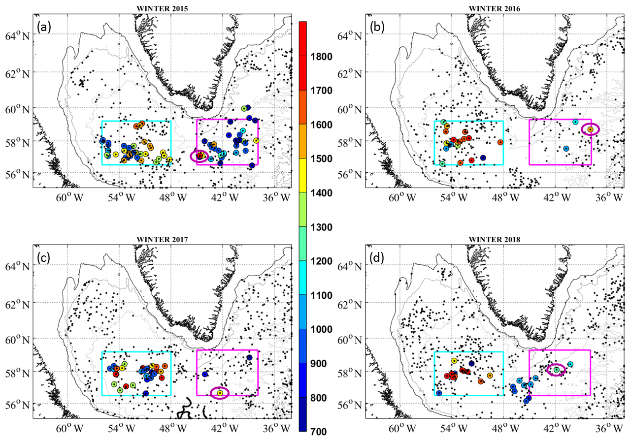
Figure 1Positions of all Argo floats north of 55∘ N in the Atlantic between 1 January and 30 April (a) 2015, (b) 2016, (c) 2017 and (d) 2018 (black and colored points). The colored points and color bar indicate the mixed layer depth (MLD) when the MLD was deeper than 700 m. The pink circles indicate the position of the maximal MLD observed SECF each winter. The pink and cyan boxes delimit the regions used for estimating the time series of atmospheric forcing and the vertical profiles of buoyancy to be removed in the SECF region and the Labrador Sea, respectively (SECF: 56.5–59.3∘ N and 45.0–38.0∘ W, Labrador Sea: 56.5–59.2∘ N and 56–48∘ W).
The convection depths that were reached in the Irminger Sea and south of Cape Farewell at the end of winter 2015 were the deepest observed in these regions since the beginning of the 21st century (de Jong et al., 2016; Piron et al., 2017, Fröb et al., 2016). In this work, we show that deep convection also happened in a region between south of Cape Farewell and the Irminger Sea (the pink box in Fig. 1) every winter from 2016 to 2018. Hereinafter, we will refer to this region as southeast Cape Farewell (SECF). We investigated the respective role of atmospheric forcing (air–sea buoyancy flux) and preconditioning (ocean interior buoyancy content) in setting the convection intensity. We also disentangled the relative contribution of salinity and temperature anomalies to the preconditioning. The paper is organized as follows. The data are described in Sect. 2. The methodology is explained in Sect. 3. We present our results in Sect. 4 and discuss them in Sect. 5. Conclusions are listed in Sect. 6.
We used temperature (T), salinity (S) and pressure (P) data measured by Argo floats north of 55∘ N in the Atlantic Ocean. These data were collected by the International Argo Program (http://www.argo.ucsd.edu/, last access: 9 January 2020; http://www.jcommops.org/, last access: 9 January 2020) and downloaded from the Coriolis Data Center (http://www.coriolis.eu.org/, last access: 9 January 2020). Only data flagged as good (quality control < 3; Argo Data Management Team, 2017) were considered in our analysis. Potential temperature (θ), density (ρ) and potential density anomaly referenced to the surface and 1000 dbar (σ0 and σ1, respectively) were estimated from T, S and P data using TEOS-10 (http://www.teos-10.org/, last access: 9 January 2020).
We used two different gridded products of ocean T and S: ISAS and EN4. ISAS (Gaillard et al., 2016; Kolodziejczyk et al., 2017) is produced by optimal interpolation of in situ data. It provides monthly fields at 152 depth levels and at 0.5∘ resolution from 2002 to 2015. Near-real-time data are also available for 2016 and 2018. EN4 (Good et al., 2013) is an optimal interpolation of in situ data; it provides monthly T and S at 1∘ spatial resolution and at 42 depth levels for the period 1900 to present.
Net air–sea heat flux (Q, the sum of radiative and turbulent fluxes), evaporation (E), precipitation (P), wind stress (τx and τy) and sea surface temperature (SST) data were obtained from the ERA-Interim reanalysis (Dee et al., 2011). ERA-Interim provides data with a time resolution of 12 h and a spatial resolution of 0.75∘. The air–sea freshwater flux (FWF) was estimated as E–P.
We used monthly absolute dynamic topography (ADT), which was computed from the daily 0.25∘ resolution ADT data provided by CMEMS (Copernicus Marine and Environment Monitoring Service, http://www.marine.copernicus.eu, last access: 9 January 2020).
3.1 Quantification of deep convection
We characterized the convection in the SPNA in the winters of 2015–2018 by estimating the mixed layer depths (MLDs) for all Argo profiles collected in the SPNA north of 55∘ N from 1 January to 30 April of each year (Fig. 1). The MLD was estimated as the shallowest of the three MLD estimates obtained by applying the threshold method of de Boyer Montégut et al. (2004) to θ, S and ρ profiles separately. The threshold method computes the MLD as the depth at which the difference between the surface (30 m) and deeper levels in a given property is equal to a given threshold. In the case that visual inspection of the winter profiles showed a thin stratified layer at the surface, a slightly deeper level (< 150 m) was considered the surface reference level. Following Piron et al. (2017), this threshold was taken as equal to 0.01 kg m−3 for ρ. For θ and S, we selected thresholds of 0.1∘ C and 0.012, respectively, because they correspond to the threshold of 0.01 kg m−3 in ρ. The latter was previously shown to perform well in the subpolar gyre on density profiles (Piron et al., 2016). The criteria for temperature and salinity were chosen to perform well when temperature and salinity anomalies within the density-defined mixed layer are density-compensated. Our MLD estimates are comparable to those obtained using MLD determination based on the Pickart et al. (2002) methods (see Sect. S1 and Figs. S1 and S2 in the Supplement).
In this paper, deep convection is characterized by profiles with an MLD deeper than 700 m (colored points in Fig. 1) because it is the minimum depth that should be reached for renewing Labrador Sea Water (LSW) (Yashayaev et al., 2007; Piron et al., 2016). The winter MLD and the associated θ, S and ρ properties were examined for the Labrador Sea and the SECF region by considering the profiles inside the cyan and pink boxes in Fig. 1, respectively. Those two boxes were defined to include all Argo profiles with an MLD deeper than 700 m during 2016–2018 and the minimum of the monthly ADT for either the SECF region or the Labrador Sea. No deep MLD was recorded in the northernmost part of the Irminger Sea during this period. We computed the maximum MLD and the MLD third quartile (Q3) from profiles with an MLD greater than 700 m in each of the two boxes separately. Q3 is the MLD value that is exceeded by 25 % of the profiles and is equivalent to the aggregate maximum depth of convection defined by Yashayaev and Loder (2016). Hereafter, we refer to Q3 as the aggregate maximum depth of convection. The properties (ρ, θ and S) of the mixed layers were defined for each winter as the vertical mean from 200 m to the MLD of all profiles with an MLD deeper than 700 m. For further use, we define the deep convection period as follows. For a given winter, the deep convection period begins the day when the first profile with a deep (> 700 m) mixed layer is detected and ends the day of the last detection of a deep mixed layer.
3.2 Time series of atmospheric forcing
The air–sea buoyancy flux (Bsurf) was calculated as the sum of the contributions of Q and FWF (Gill, 1982; Billheimer and Talley, 2013):
where α and β are the coefficients of thermal and saline expansions, respectively, estimated from surface T and S. The gravitational acceleration g is equal to 9.8 m s−2, the reference density of sea water ρ0 is equal to 1026 kg m−3 and the heat capacity of sea water Cp is equal to 3990 J kg −1 ∘C−1. SSS is the sea surface salinity (Q: W m−2, FWF: m s−1).
For easy comparison with previous results, which only considered the heat component of the buoyancy air–sea flux (e.g., Yashayaev and Loder, 2017; Piron et al., 2017; Rhein et al., 2017), Bsurf (m2 s−3) was converted (W m−2) following Eq. (2) and noted :
The FWF was also converted (W m−2) using
We also computed the horizontal Ekman buoyancy flux (BFek), which can be decomposed into the horizontal Ekman heat flux (HFek) and salt flux (SFek).
BFek=SFek – HFek. Ue and Ve are the eastward and northward components of the Ekman horizontal transport estimated from the wind stress meridional and zonal components. SSD, SST and SSS are ρ, T and S at the surface of the ocean (BFek, HFek and SFe: J s−1 m−2). Because ERA-Interim does not supply SSD or SSS, they were estimated from EN4 as follows. The monthly T and S data at 5 m of depth from EN4 were interpolated on the same time and space grid as the air–sea fluxes from ERA-Interim (12 h and 0.75∘, respectively). SSD was estimated from those interpolated EN4 data (SST and SSS). Properties at 5 m of depth were considered to be representative of the Ekman layer. Data at locations where the ocean bottom was shallower than 1000 m were excluded from the analysis to avoid regions covered by sea ice.
Following Piron et al. (2016), the time series of atmospheric forcing were estimated for the SECF region and the Labrador Sea as follows. First, the gridded air–sea flux data and the horizontal Ekman fluxes were averaged over the pink (SECF region) and cyan (Labrador Sea) boxes (Fig. 1). Second, we estimated the accumulated fluxes from 1 September to 31 August the year after. Finally, we computed the time series of the anomalies of the accumulated fluxes from 1 September to 31 August with respect to the 1993–2016 mean.
Finally, in order to quantify the net intensity of the atmospheric forcing over the winter, we computed estimates of fluxes accumulated from 1 September to 31 March the year after. Following Piron et al. (2017), the associated errors were calculated by a Monte Carlo simulation using 50 random perturbations of Q, FWF and Bsurf. The error amounted to 0.05, 0.04 and 0.03 J m−2 for , Q and FWF*, respectively. The error of the horizontal Ekman buoyancy transport was also estimated by a Monte Carlo simulation and amounted to 0.04 J m−2.
3.3 Preconditioning of the water column
The preconditioning of the water column was evaluated as the buoyancy that has to be removed (B(zi)) from the late summer density profile to homogenize it down to a depth zi:
where σ0(z) is the vertical profile of potential density anomaly estimated from the profiles of T and S measured by Argo floats in September in the given region (pink or cyan box in Fig. 1).
Following Schmidt and Send (2007), we split B into a temperature (Bθ) and salinity (BS) term:
In order to compare the preconditioning with the heat to be removed and/or air–sea heat fluxes, B, Bθ and BS are reported in Joules per square meter. B, Bθ and BS were estimated for a given year from the mean of all September profiles of B, Bθ and BS. The associated errors were estimated as , where n is the number of profiles used to compute the September mean values.
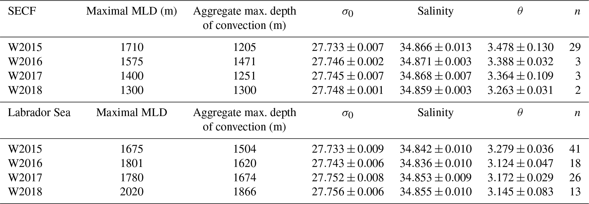
Table 1Properties of the deep convection SECF and in the Labrador Sea in winters 2015–2018. We show: the maximal MLD observed, the aggregate maximum depth of convection, the σ0, S and θ of the winter mixed layer formed during the convection event and n, which is the number of Argo profiles indicating deep convection. The uncertainties given with σ0, S and θ are the standard deviation of the n values considered to estimate the mean values.
4.1 Intensity of deep convection and properties of newly formed LSW
We examine the time evolution of the winter mixed layer SECF since the exceptional convection event of winter 2015 (W2015 hereinafter) (Table 1 and Figs. 1–3). In W2015, we recorded a maximum MLD of 1710 m south of Cape Farewell (Fig. 1a), in line with Piron et al. (2017). The maximum MLD of 1575 m observed for W2016 (Fig. 1b) is compatible with the active mixed layer > 1500 m observed in a mooring array in the central Irminger Sea by de Jong et al. (2018). For W2015 and W2016, the aggregate maximum depth of convection was 1205 and 1471 m, respectively (Table 1). In W2017, deep convection was observed from three Argo profiles (Figs. 1c and 2a–c). The maximum MLD of 1400 m was observed on 16 March 2017 at 56.65∘ N–42.30∘ W. In W2018, the maximum MLD of 1300 m was observed on 24 February at 58.12∘ N, 41.84∘ W (Figs. 1d, 2d–f). Float 5903102 measured an MLD of 1100 m south of Cape Farewell (Fig. 1d), but the estimated MLDs coincided with the deepest levels of measurement of the float so that these estimates, possibly biased low (see Fig. 2d–f), were discarded from our analysis. These results show that convection deeper than 1300 m occurred during four consecutive winters SECF.
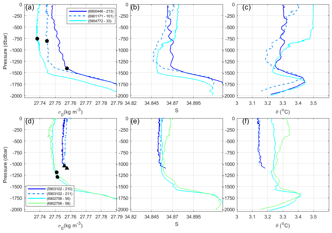
Figure 2Vertical distribution of σ0, S and θ of Argo profiles showing an MLD deeper than 700 m SECF in winter 2017 (a, b, c) and in winter 2018 (d, e, f). The black points indicate the MLD. The triangles in (d) are the MLD that coincided with the maximal profiling pressure reached by the float. In the legend, the float and cycle of each profile are indicated.
Although the number of floats showing deep convection in W2017 and W2018 was small (three and two floats, respectively), it represented a significant percentage of the floats operating in the SECF box at that time. The percentage of floats showing deep convection in the SECF region was computed for the deep convection periods defined from 15 January to 21 April 2015, 22 February to 21 March 2016, 16 March to 4 April 2017 and 24 February to 26 March 2018. The longest period of deep convection occurred in W2015 and the shortest in 2017. The percentages of floats showing deep convection during the deep convection period are 73 %, 50 %, 33 % and 50 % for the winters of 2015, 2016, 2017 and 2018, respectively. The lowest percentage is found for W2017, but it is still substantial. It might reflect the fact that for this specific year floats showing a deep MLD were found in the southwestern corner of the SECF box only, suggesting that convection did not occur over the full box.
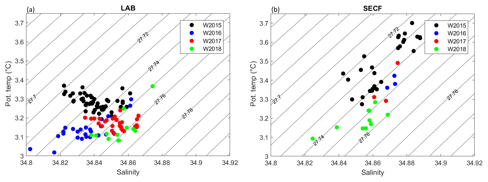
Figure 3TS diagrams in the mixed layer for profiles with an MLD deeper than 700 m during the winters of 2015, 2016, 2017 and 2018 for (a) the Labrador Sea and (b) SECF. The properties of the mixed layers were estimated as the vertical means between 200 m and the MLD.
The properties (σ0, S and θ) of the end-of-winter mixed layer were estimated for the four winters (Table 1 and Fig. 3). We observed that, between W2015 and W2018, the water mass formed by deep convection significantly densified and cooled by 0.019 kg m−3 and 0.215 ∘C, respectively (see Table 1 and Fig. 3).
In the Labrador Sea, the aggregate maximum depth of convection increased from 2015 to 2018 (see Table 1). Deep convection observed in the Labrador Sea in W2018 was the most intense since the beginning of the Argo era (see Fig. 2c in Yashayaev and Loder, 2016). From W2015 to W2018, newly formed LSW cooled, became saltier, and densified by 0.134 ∘C, 0.013 and 0.023 kg m−3, respectively (Table 1).
The water mass formed SECF is warmer and saltier than that formed in the Labrador Sea (Fig. 3). The deep convection SECF is always shallower than in the Labrador Sea. This result is discussed later in Sect. 5.
4.2 Analysis of the atmospheric forcing southeast of Cape Farewell
The seasonal cycles of and Q are in phase and of the same order of magnitude, while FWF*, which is positive and 1 order of magnitude lower than Q, does not present a seasonal cycle (Fig. S3). The means (1993–2018) of the cumulative sums from 1 September to 31 March of Q, FWF* and estimated over the SECF box (Fig. 1) are , and J m−2, respectively. is 10 % lower on average than Q because of the buoyancy addition by FWF*. Considering the Ekman transports, the 1993–2018 means of the accumulated BFek, HFek and SFek from 1 September to 31 March amount to , and J m−2, respectively. The horizontal Ekman heat flux is negative, while the Ekman buoyancy flux is positive. This buoyancy gain indicates a southeastward transport of surface freshwater caused by dominant winds from the southwest. It is noteworthy that BFek is 1 order of magnitude smaller than the .
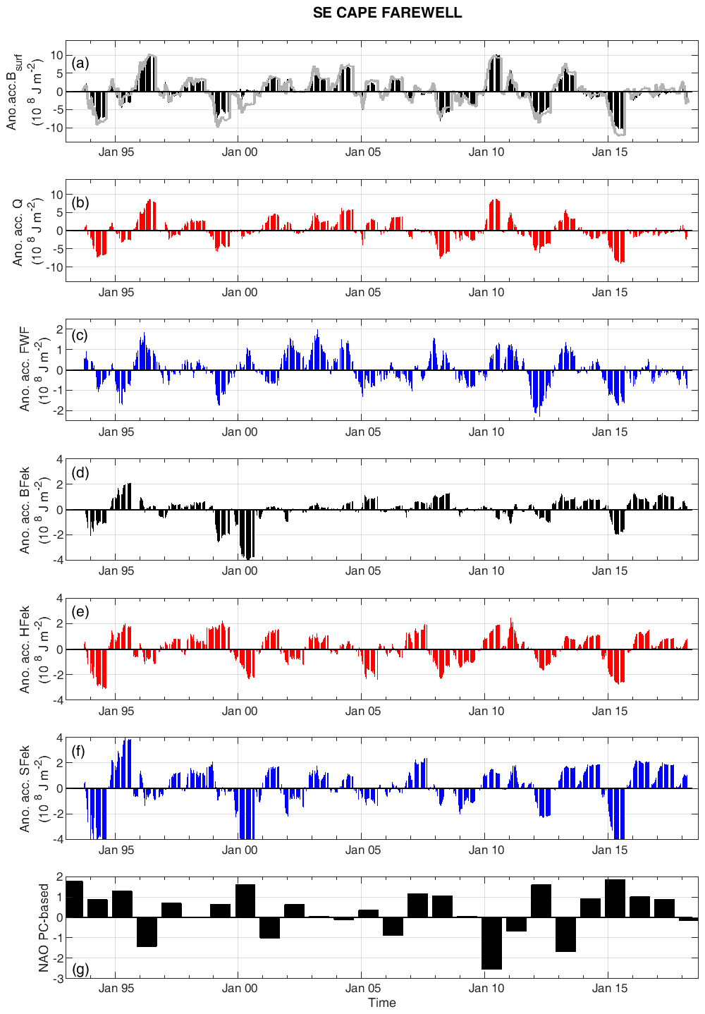
Figure 4Time series of anomalies of accumulated (a) , (b) Q, (c) FWF* (d) BFek, (e) HFek and (f) SFek averaged in the SECF region. They are anomalies with respect to 1993–2016. The accumulation was from 1 September to 31 August the following year. The winter North Atlantic Oscillation (NAO) index (Hurrell et al., 2018) is also represented in (g). The gray line in (a) is the sum of the anomalies of accumulated and BFek. Note that the range of values in the y axis is not the same in all the plots.
The total atmospheric forcing SECF was quantified as the sum of and BFek. The anomalies of accumulated fluxes from 1 September to 31 August the year after, with respect to the mean 1993–2016, are displayed in Fig. 4 for the SECF box. The gray line in Fig. 4a is the total atmospheric forcing anomaly ( plus BFek). We identify years with very negative buoyancy loss in the SECF region, e.g., 1994, 1999, 2008, 2012 and 2015. The very negative anomalies of atmospheric forcing in 1999 and 2015 were caused by the very negative anomalies in both (Fig. 4a) and BFek (Fig. 4d). This correlation was not observed for all the years presenting a negative anomaly of atmospheric forcing. It is noteworthy that during W2016, W2017 and W2018, the anomaly of atmospheric forcing was close to zero.
Contrary to the very negative anomaly in atmospheric fluxes over the SECF region observed for W2015, the atmospheric fluxes were close to the mean during W2016, W2017 and W2018.
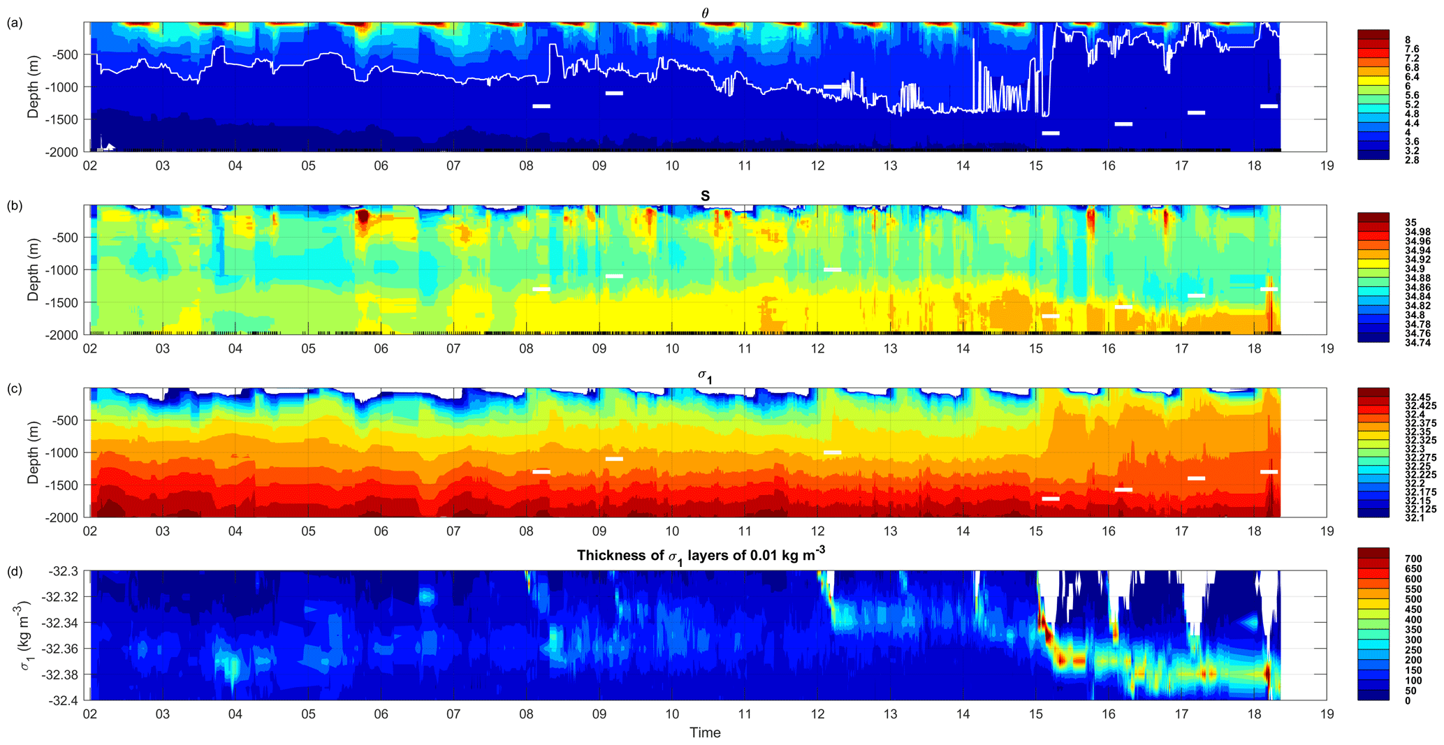
Figure 5Time evolutions of vertical profiles measured from Argo floats in the SECF region: (a) θ, (b) S, (c) σ1 and (d) the thickness of 0.01 kg m−3 thick σ1 layers. The white horizontal bars in plots (a), (b) and (c) indicate the maximal convection depth observed in the Irminger Sea or SECF when deep convection occurred. The white line in plot (a) indicates the depth of the isotherm 3.6 ∘C. The black vertical ticks on the x axes of plot (b) indicate times of Argo measurements. These figures were created from all Argo profiles reaching deeper than 1000 m in the SECF region (56.5–59.3∘ N, 45–38∘ W; pink box in Fig. 1). The yearly numbers of Argo profiles used in this figure are shown in Fig. S5.
4.3 Analysis of the preconditioning of the water column southeast of Cape Farewell
Our hypothesis is that the exceptional deep convection that happened in W2015 in the SECF region favorably preconditioned the water column for deep convection the following winters. The time evolutions of θ, S, σ1 and Δσ1=0.01 kg m−3 layer thicknesses (Fig. 5) show a marked change in the hydrographic properties of the SECF region at the beginning of 2015 caused by the exceptional deep convection that occurred during W2015 (see Piron et al., 2017). The intermediate waters (500–1000 m) became colder than the years before, and despite a slight decrease in salinity, the cooling caused the density to increase (Fig. 5c). Figure 5d shows Δσ1=0.01 kg m−3 layer thicknesses larger than 600 m appearing at the end of W2015 for the first time since 2002. In the density range 32.36–32.39 kg m−3, these layers remained thicker than ∼450 m during W2016 to W2018. This indicates low stratification at intermediate depths and a favorable preconditioning of intermediate waters for deep convection initiated by W2015 deep convection. The denser density of the core of the thick layers in 2017–2018 compared with 2015–2016 agrees with the densification of the mixed layer SECF shown in Table 1 and Fig. 3.
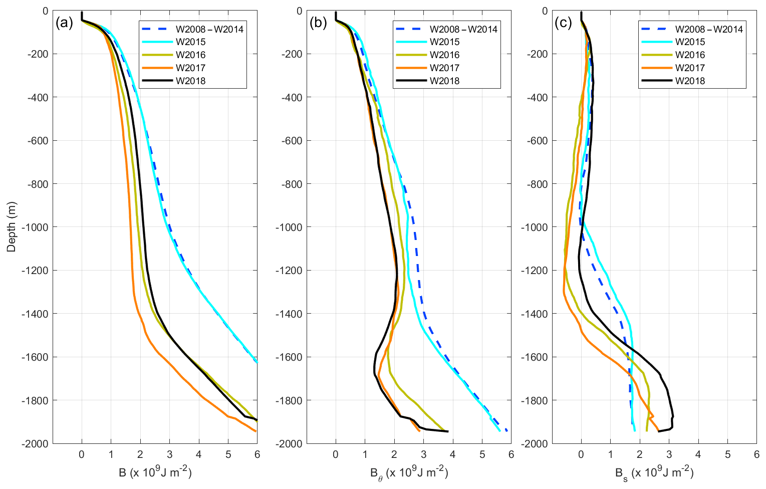
Figure 6Vertical profile of (a) the buoyancy to be removed (B), (b) the thermal component (Bθ) and (c) the salinity component (BS). They were calculated from all Argo data measured in the SECF box (see Fig. 1) in September before the winter indicated in the legend. For W2015 and W2018, we considered data from 15 August to 30 September 2017 because not enough data were available in September. The number of Argo profiles taken into account to estimate the B profiles was more than 10 for all the winters.
B(zi) is our estimate of the preconditioning of the water column before winter (see the Methods section). Figure 6a shows that, deeper than 100 m, B for W2016, W2017 and W2018 was smaller than B for W2015 or B for the mean W2008–W2014. Furthermore, for W2016, W2017 and 2018, B remained nearly constant with depth between 600 and 1300 m, which means that once the water column has been homogenized down to 600 m, little additional buoyancy loss results in the homogenization of the water column down to 1300 m. Both conditions, (i) less buoyancy to be removed and (ii) the absence of a gradient in the B profile down to 1300 m, indicate a more favorable preconditioning of the water column for W2016, W2017 and W2018 than during W2008–W2015.
To understand the relative contributions of θ and S to the preconditioning, we computed the thermal (Bθ) and haline (BS) components of B (). In general, Bθ (BS) increases with depth when θ decreases (S increases) with depth. On the contrary, a negative slope in a Bθ (BS) profile corresponds to θ increasing (S decreasing) with depth and is indicative of a destabilizing effect. The negative slopes in Bθ and BS profiles are not observed simultaneously because density profiles are stable.
We describe the relative contributions of Bθ and BS to B by looking first at the mean 2008–2014 profiles (discontinuous blue lines in Fig. 6). Bθ accounts for most of the increase in B from the surface to 800 m and below 1400 m (see Fig. 6a and b). The negative slope in the BS profile between 800 and 1000 m (Fig. 6c) slightly reduces B (Fig. 6a) and is due to the decrease in S associated with the core of LSW (see Fig. 3 in Piron et al., 2016). In the layer 1000–1400 m, the increase in B (Fig. 6a) is mainly explained by the increase in BS (Fig. 6c), which follows the increase in S in the transition from LSW to Iceland Scotland Overflow Water (ISOW). This transition layer will be referred to hereinafter as the deep halocline. The preconditioning of the water column is usually analyzed in terms of heat (e.g., Piron et al., 2015, 2017). The decomposition of B in Bθ and BS reveals that θ governs B in the layer 0–800 m. S tends to reduce the stabilizing effect of θ in the layer 800–1000 m and reinforces it in the layer 1000–1400 m by adding up to 1×10⁹ J m2 to B.
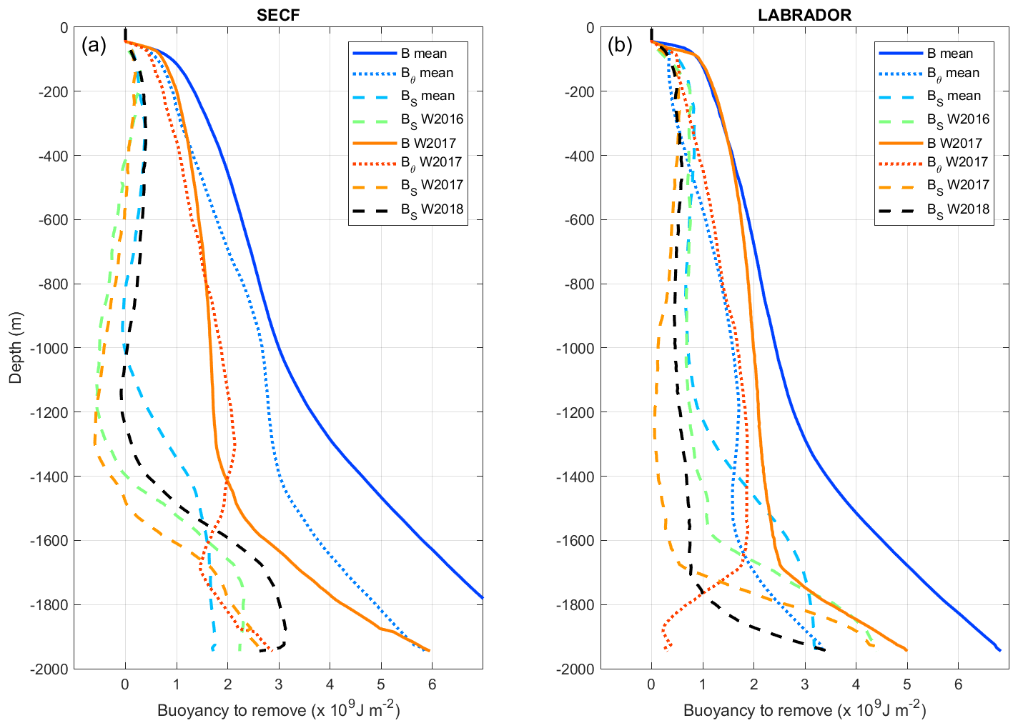
Figure 7Decomposition of the profiles of buoyancy to be removed (B, continuous lines) in its thermal (Bθ, dotted lines) and salinity (BS, dashed lines) components in (a) the SECF region; (b) the Labrador Sea. The BS components for W2016 and W2018 were added to show the evolution of the depth of the deep halocline.
In order to further understand why the SECF region was favorably preconditioned during the winters of 2016–2018, we compare the Bθ and BS of W2017, which was the most favorably preconditioned winter, with the mean 2008–2014 (Fig. 7a). From the surface to 1600 m, Bθ and BS were smaller for W2017 than for the mean 2008–2014. There are two additional remarkable features. First, in the layer 500–1000 m, the large reduction of Bθ compared to the 2008–2014 mean mostly explains the decrease in B in this layer. Second, the more negative value of BS in the layer 1100–1300 m, compared to the 2008–2014 mean, eroded the Bθ slope, making the B profile more vertical for W2017 than for the mean. The more negative contribution of BS in the layer 1100–1300 m comes from the fact that the deep halocline was deeper for W2017 (1300 m; see orange dashed line in Fig. 7a) than for the mean 2008–2014 (1000 m; see blue dashed line in Fig. 7a). Finally, we note that the profiles of B(zi), Bθ(zi) and BS(zi) for W2016 and W2018 are more similar to the profiles of W2017 than to those of W2015 or to the mean 2008–2014 (see Fig. 6), which indicates that the water column was also favorably preconditioned for deep convection in W2016 and W2018 for the same reasons as in W2017.
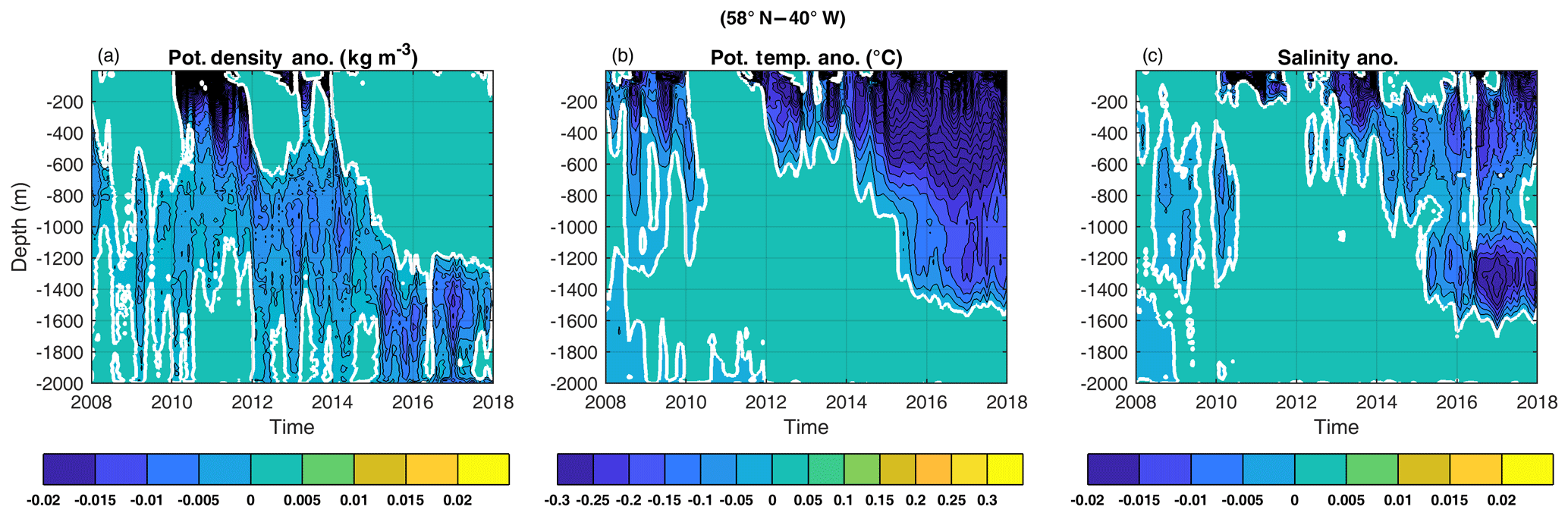
Figure 8Evolution of vertical profiles of monthly anomalies of (a) σ0, (b) θ and (c) S at 58∘ N, 40∘ W. The anomalies were estimated from the ISAS database (Gaillard et al., 2016) and were referenced to the monthly mean estimated for 2002–2016.
The origin of the changes in B is now discussed from the time evolutions of the monthly anomalies of θ, S and σ0 at 58∘ N–40∘ W, which is at the center of the SECF box (Fig. 8). The time evolutions there are similar to those at any other location inside the SECF box. These anomalies were computed using ISAS Gaillard et al., 2016) and were referenced to the monthly mean of 2002–2016. A positive anomaly of σ0 appeared in 2014 between the surface and 600 m (Fig. 8a) and reached 1200 m in 2015 and beyond. This positive anomaly of σ0 correlates with a negative anomaly of θ. The latter, however, reached ∼1400 m of depth in 2016, which is deeper than the positive anomaly of σ0. The negative anomaly of S between 1000 and 1500 m that appeared in 2015 and strongly reinforced in 2016 caused the negative anomaly in σ0 between 1200 and 1500 m (the density anomaly caused by the negative anomaly in θ between 1200 and 1400 m does not balance the density anomaly caused by the negative anomaly of S).
The θ and S anomalies in the water column during 2016–2018 explain the anomalies of B, Bθ and BS and can be summarized as follows. On the one hand, the properties of the surface waters (down to 500 m) were colder than previous years and, despite the fact that they were also fresher, they were denser. The density increase in the surface water reduced the density difference with the deeper-lying waters. The intermediate layer (500–1000 m) was also favorably preconditioned due to the observed cooling. Additionally, in the layer 1100–1300 m, the large negative anomaly of BS with respect to its mean is explained by the decrease in S in this layer, which caused a decrease in σ0 and consequently reduced the σ0 difference with the shallower-lying water. The decrease in S also resulted in a deepening of the deep halocline.

Figure 9Horizontal distribution of the anomalies of S (a, b, c), θ (d, e, f) and σ0 (g, h, i) in the layer 1200–1400 m in February 2015 (a, d, g), February 2016 (b, e, h) and February 2017 (c, f, i). The monthly anomalies were estimated from the ISAS database and were referenced to the period 2002–2016.
4.4 Atmospheric forcing versus preconditioning of the water column
We now use the estimates of the accumulated atmospheric forcing () from 1 September to 31 March the year after (see Fig. S4) to predict the maximum convection depth for a given winter based on September profiles of B. The predicted convection depth is determined as the depth at which B(zi) (Fig. 6a) equals the accumulated atmospheric forcing. The associated error was estimated by propagating the error in the atmospheric forcing (0.05×10⁹ J m−2). The accumulated atmospheric forcing amounted to , and J m−2 for W2015, W2016, W2017 and W2018, respectively. We found predicted convection depths of 1085±20, 1285±20, 1415±20 and 345±20 m for W2015, W2016, W2017 and W2018, respectively. We consider the aggregate maximum depth of convection to be the observed estimate of the MLD (Table 1). The predicted MLD agrees with the observed MLD within ±200 m. The differences could be due to errors in the atmospheric forcing (Josey et al., 2018), lateral advection and/or spatial variation in the convection intensity within the box not captured by the Argo sampling.
The satisfactory predictability of the convection depth with our 1-D model indicates that deep convection occurred locally. In spite of the fact that the atmospheric forcing was close to mean (1993–2016) conditions during W2016, W2017 and W2018, convection depths > 1300 m were reached in the SECF region. This was only possible thanks to the favorable preconditioning.
Deep convection happens in the Irminger Sea and south of Cape Farewell during specific winters characterized by a strong atmospheric forcing (high buoyancy loss), a favorable preconditioning (low stratification) or both at the same time (Bacon et al., 2003; Pickart et al., 2003). In the Irminger Sea, strong atmospheric forcing explained, for instance, the very deep convection (reaching depths greater than 1500 m) observed in the early 1990s (Pickart et al., 2003) and in W2015 (de Jong et al. 2016; Fröb et al., 2016; Piron et al., 2017). It also explained the return of deep convection in W2008 (Väge et al., 2009) and in W2012 (Piron et al., 2016). The favorable preconditioning caused by the densification of the mixed layer during W2008 favored a new deep convection event in W2009 despite neutral atmospheric forcing (de Jong et al., 2012). Similarly, the preconditioning observed after W2015 in the SECF region favored deep convection in W2016 (this work). The favorable preconditioning persisted for three consecutive winters (2016–2018) in the SECF region, which allowed deep convection although atmospheric forcing was close to the climatological values. Why did this favorable preconditioning persist in time?
We previously showed that during 2016–2018 two hydrographic anomalies affected different ranges of the water column in the SECF box: a cooling intensified in the layer 200–800 m and a freshening intensified in the 1000–1500 m layer. Those resulted in a decrease in the vertical density gradient between the intermediate and the deeper layers, creating a favorable preconditioning of the water column. Note that the cooling affected the layer from the surface to 1400 m, and the freshening affected the layer from the near surface to 1600 m, but the cooling and the freshening were intensified at different depth ranges (Fig. 8).
We see in Fig. 5a a sudden decrease in θ in the intermediate layers in 2015 compared to the previous years. It indicates that the decrease in θ of the intermediate layer likely originated locally during W2015 when extraordinary deep convection happened. A slight freshening of the water column (400–1500 m) appeared in 2015, likely caused by the W2015 convection event; then it decreased before a second S anomaly intensified in 2016 between 1100 and 1400 m (Fig. 8c). It is unlikely that this second anomaly was exclusively locally formed by deep convection because it intensified during summer 2016. Our hypothesis is that this second S anomaly originated in the Labrador Sea and was further transferred to the SECF region by the cyclonic circulation encompassing the Labrador Sea and Irminger Sea at these depths (Daniault et al., 2016; Ollitrault and Colin de Verdière, 2014; Lavander et al., 2000; Straneo et al., 2003). This is corroborated by the 2-D evolution of the anomalies in S in the layer 1200–1400 m (Fig. 9): a negative anomaly in S appeared in the Labrador Sea in February 2015, which was transferred southward and northeastward in February 2016 and intensified over the whole SPNA in February 2017. By this mechanism, the advection from the Labrador Sea contributed to create property anomalies in the water column. However, the buoyancy budget showed that this was a minor contribution compared to the buoyancy loss due to the local air–sea flux, even if it was essential to preconditioning the water column for deep convection.
We now compare the atmospheric forcing and the preconditioning of the water column in the SECF region with those of the nearby Labrador Sea where deep convection happens almost every year. The atmospheric forcing over the Labrador Sea is ∼15 % larger than that over the SECF region: the means (1993–2018) of the atmospheric forcing, defined as the time-accumulated from 1 September to 31 March the year after, are J m−2 in the Labrador Sea and J m−2 in the SECF region. The difference was larger during the period 2016 – 2018 when the atmospheric forcing equaled J m−2 in the Labrador Sea and J m−2 in the SECF region. In terms of preconditioning, the 2008–2014 mean B profile (blue continuous lines in Fig. 7) was lower by J m−2 in the Labrador Sea than SECF for the surface to the 1000 m layer and by more than 1×10⁹ J m−2 below 1200 m. This indicates that the water column was more favorably preconditioned in the Labrador Sea than in the SECF region during 2008–2014. Differently, B for W2017 shows slightly lower values from the surface to 1300 m in the SECF region than in the Labrador Sea (see orange lines in Fig. 7). However, B in the Labrador Sea remains constant down to the depth of the deep halocline between LSW and North Atlantic Deep Water (NADW) at 1700 m. In the SECF region, the deep halocline remained at ∼1300 m between 2016 and 2018 (see BS lines in Fig. 7a). Differently, in the Labrador Sea, the deep halocline deepened from 1200 m for the mean to 1735, 1775 and 1905 m in W2016, W2017 and W2018, respectively (see the dashed lines in Fig. 7b). The deep halocline acts as a physical barrier for deep convection in both the SECF region and the Labrador Sea, but because the deep halocline is deeper in the Labrador Sea than in the SECF region, the preconditioning is more favorable to a deeper convection in the Labrador Sea than in the SECF region. Summarizing, in the winters of 2016–2018 in the Labrador Sea, both atmospheric forcing and preconditioning of the water column allowed for the deepest convection depth in the Labrador Sea since the beginning of the Argo period (comparison of our results with those of Yashayaev and Loader, 2017). In contrast, in the SECF region during the same period, the atmospheric forcing was close to climatological values, and the favorable preconditioning of the water column allowed for 1300 m of depth convection, which was exceptional for the SECF region.
The Labrador Sea, SECF region and Irminger Sea are three distinct deep convection sites (e.g., Yashayaev et al., 2007; Bacon et al., 2003; Pickart et al., 2003; Piron et al., 2017). In this work, we give new insights on the connections between the different sites, showing how the lateral advection of fresh LSW formed in the Labrador Sea favored the preconditioning in the SECF region, fostering deeper convection.
Climate models forecast an increasing input of freshwater in the North Atlantic due to ice melting under present climate change (Bamber et al., 2018), which could reduce or even shut down the deep convection in the North Atlantic (Yang et al., 2016; Brodeau and Koenigk, 2016). We observed a fresh anomaly in the surface waters in regions close to the eastern coast of Greenland in 2016 that extended to the whole Irminger Sea in 2017 (Fig. S6). However, this surface freshening did not hamper the deep convection in the SECF region, possibly because the surface water also cooled. Swingedouw et al. (2013) indicated that the freshwater signal due to Greenland ice sheet melting is mainly accumulating in the Labrador Sea. However, no negative anomaly of S was detected in the surface waters of the Labrador Sea (Fig. S6). It might be explained by the intense deep convection affecting the Labrador Sea since 2014 that could have transferred the surface freshwater anomaly to the ocean interior. This suggests that, in the last years, the interactions between expected climate change anomalies and the natural dynamics of the system combined to favor very deep convection. This, however, does not foretell the long-term response to climate change.
During 2015–2018 winter deep convection happened in the SECF region, reaching deeper than 1300 m. The deep convection of W2015 was observed over a larger region and during a longer period of time than the deep convection events of the winters of 2016, 2017 and 2018. Despite these differences, it is the first time that deep convection, with a maximum convection depth greater than 1300 m, was observed in this region during four consecutive winters.
The atmospheric forcing and preconditioning of the water column were evaluated in terms of buoyancy. We showed that the atmospheric forcing is 10 % weaker when evaluated in terms of buoyancy than in terms of heat because of the non-negligible effect of the freshwater flux. The analysis of the preconditioning of the water column in terms of buoyancy to be removed (B) and its thermal and salinity terms (Bθ and BS) revealed that Bθ dominated the B profile from the surface to 800 m, and BS reduced the B in the 800–1000 m layer because of the low salinity of LSW. Deeper, BS increased B due to the deep halocline (LSW–ISOW) that acted as a physical barrier limiting the depth of the convection.
During 2016–2018, the air–sea buoyancy losses were close to the climatological values, and very deep convection was possible thanks to the favorable preconditioning of the water column. It was surprising that these events reached convection depths similar to those observed in W2012 and W2015, when the latter were caused by high air–sea buoyancy loss intensified by the effect of strong wind stress. It was also surprising that the water column remained favorably preconditioned during three consecutive winters without strong atmospheric forcing. In this paper, we studied the reasons why this happened.
The preconditioning for deep convection during 2016–2018 was particularly favorable due to the combination of two types of hydrographic anomalies affecting different depth ranges. First, the surface and intermediate waters (down to 800 m) were favorably preconditioned because buoyancy (density) decreased (increased) due to the cooling caused by the atmospheric forcing. Second, buoyancy (density) increased (decreased) in the layer 1200–1400 m due to the decrease in S caused by the lateral advection of fresher LSW formed in the Labrador Sea. The S anomaly of this layer resulted in a deeper deep halocline. Hence, the cooling of the intermediate water was essential to reach a convection depth of 800–1000 m, and the freshening in the layer 1200–1400 m and the associated deepening of the deep halocline allowed for very deep convection (> 1300 m) in W2016–W2018.
The Argo data were collected and made freely available by the International Argo Program and the national programs that contribute to it (https://doi.org/10.17882/42182; Argo group, 2019). The ISAS data were downloaded from the SEANOE site (https://doi.org/10.17882/52367; Kolodziejczyk et al., 2017). The EN4 data are available at http://hadobs.metoffice.com/en4/download.html (Good et al., 2013). The ERA-Interim data are available at https://www.ecmwf.int/en/forecasts/datasets/reanalysis-datasets/era-interim (Dee et al., 2011). The NAO data were downloaded from the UCAR Climate Data Guide website (https://climatedataguide.ucar.edu/climate-data/hurrell-north-atlantic-oscillation-nao-index-station-based, last access: 9 January 2020; Hurrell et al., 2018). The Ssalto/Duacs altimeter products were produced and distributed by the Copernicus Marine and Environment Monitoring Service (CMEMS) (http://marine.copernicus.eu/services-portfolio/access-to-products/?option=com_csw&view=details&product_id=SEALEVEL_GLO_PHY_L4_REP_OBSERVATIONS_008_047, last access: 9 January 2020).
The supplement related to this article is available online at: https://doi.org/10.5194/os-16-99-2020-supplement.
PZ treated and analyzed the data. PZ and HM interpreted the results. PZ, HM and VT discussed the results and wrote the paper.
The authors declare that they have no conflict of interest.
We thank all the navy staff and PIs contributing to the deployment of Argo floats; without them this work would not be possible. We thank Marieke Femke de Jong and two anonymous reviewers; their comments and suggestions have enriched our work.
This paper is a contribution to the EQUIPEX NAOS project funded by the French National Research Agency (ANR) under reference ANR-10-EQPX-40.
This paper was edited by Neil Wells and reviewed by Femke de Jong and two anonymous referees.
Argo Data Management Team: Argo user's manual V3.2, https://doi.org/10.13155/29825, 2017.
Argo group: Argo float data and metadata from Global Data Assembly Centre (Argo GDAC), SEANOE, https://doi.org/10.17882/42182, 2019.
Bacon, S.: Circulation and Fluxes in the North Atlantic between Greenland and Ireland, J. Phys. Oceanogr., 27, 1420–1435, https://doi.org/10.1175/1520-0485(1997)027<1420:CAFITN>2.0.CO;2, 1997.
Bacon, S., Gould, W. J., and Jia, Y.: Open-ocean convection in the Irminger Sea, Geophys. Res. Lett., 30, 1246, https://doi.org/10.1029/2002GL016271, 2003.
Bamber, J. L., Tedstone, A. J., King, M. D., Howat, I. M., Enderlin, E. M., van den Broeke, M. R., and Noel, B.: Land Ice Freshwater Budget of the Arctic and North Atlantic Oceans: 1. Data, Methods, and Results, J. Geophys. Res.-Oceans, 123, https://doi.org/10.1002/2017JC013605, 2018.
Billheimer, S. and Talley, L. D.: Near cessation of Eighteen Degree Water renewal in the western North Atlantic in the warm winter of 2011–2012, J. Geophys. Res.-Oceans, 118, 6838–6853, https://doi.org/10.1002/2013JC009024, 2013.
Brodeau, L. and Koenigk, T.: Extinction of the northern oceanic deep convection in an ensemble of climate model simulations of the 20th and 21st centuries, Clim. Dynam., 46, 2863–2882, https://doi.org/10.1007/s00382-015-2736-5, 2016.
Centurioni and Gould, W. J.: Winter conditions in the Irminger Sea observed with profiling floats, J. Marine Res., 62, 313–336, 2004.
Daniault, N., Mercier, H., Lherminier, P., Sarafanov, A., Falina, A., Zunino, P., and Gladyshev, S.: The northern North Atlantic Ocean mean circulation in the early 21st century, Prog. Oceanogr., 146, 142–158, https://doi.org/10.1016/j.pocean.2016.06.007, 2016.
de Boyer Montégut, C., Madec, G., Fischer, A. S., Lazar, A., and Iudicone, D.: Mixed layer depth over the global ocean: An examination of profile data and a profile-based climatology, J. Geophys. Res.-Oceans, 109, 1–20, https://doi.org/10.1029/2004JC002378, 2004.
de Jong, M. F. and de Steur, L.: Strong winter cooling over the Irminger Sea in winter 2014–2015, exceptional deep convection, and the emergence of anomalously low SST, Geophys. Res. Lett., 43, 7106–7113, https://doi.org/10.1002/2016GL069596, 2016.
de Jong, M. F., Van Aken, H. M., Våge, K., and Pickart, R. S.: Convective mixing in the central Irminger Sea: 2002–2010, Deep-Sea Res. Pt. I, 63, 36–51, https://doi.org/10.1016/j.dsr.2012.01.003, 2012.
de Jong, M. F., Oltmanns, M., Karstensen, J., and de Steur, L.: Deep Convection in the Irminger Sea Observed with a Dense Mooring Array, Oceanography, 31, 50–59, https://doi.org/10.5670/oceanog.2018.109, 2018.
Dee, D. P., Uppala, S. M., Simmons, A. J., Berrisford, P., Poli, P., Kobayashi, S., and Vitart, F.: The ERA-Interim reanalysis: Configuration and performance of the data assimilation system, Q. J. Roy. Meteor. Soc., 137, 553–597, https://doi.org/10.1002/qj.828, 2011 (data available at: https://www.ecmwf.int/en/forecasts/datasets/reanalysis-datasets/era-interim, last access: 9 January 2020).
Fröb, F., Olsen, A., Våge, K., Moore, G. W. K., Yashayaev, I., Jeansson, E., and Rajasakaren, B.: Irminger Sea deep convection injects oxygen and anthropogenic carbon to the ocean interior, Nat. Commun., 7, 13244, https://doi.org/10.1038/ncomms13244, 2016.
Gaillard, F., Reynaud, T., Thierry, V., Kolodziejczyk, N., and Von Schuckmann, K.: In situ-based reanalysis of the global ocean temperature and salinity with ISAS: Variability of the heat content and steric height, J. Climate, 29, 1305–1323, https://doi.org/10.1175/JCLI-D-15-0028.1, 2016.
Gill, A. E.: Atmosphere-Ocean Dynamics, vol. 30, Academic, San Diego, CA, 1982.
Good, S. A., Martin, M. J., and Rayner, N. A.: EN4: Quality controlled ocean temperature and salinity profiles and monthly objective analyses with uncertainty estimates, J. Geophys. Res.-Oceans, 118, 6704–6716, https://doi.org/10.1002/2013JC009067, 2013 (data available at: http://hadobs.metoffice.com/en4/download.html, last access: 9 January 2020).
Hurrell, J. and National Center for Atmospheric Research Staff (Eds.): The Climate Data Guide: Hurrell North Atlantic Oscillation (NAO) Index (station-based), available at: https://climatedataguide.ucar.edu/climate-data/hurrell-north-atlantic-oscillation-nao-index-station-based (last access: 28 June 2018), 2018.
Josey, S. A., Hirschi, J. J.-M., Sinha, B., Duchez, A., Grist, J. P., and Marsh, R.: The Recent Atlantic Cold Anomaly: Causes, Consequences, and Related Phenomena, Annu. Rev. Mar. Sci., 10, 475–501, https://doi.org/10.1146/annurev-marine-121916-063102, 2018.
Kieke, D. and Yashayaev, I.: Studies of Labrador Sea Water formation and variability in the subpolar North Atlantic in the light of international partner and collaboration, Prog. Oceanogr., 132, 220–232, https://doi.org/10.1016/j.pocean.2014.12.010, 2015.
Kolodziejczyk, N., Prigent-Mazella, A., and Gaillard, F.: ISAS-15 temperature and salinity gridded fields, Seanoe, https://doi.org/10.17882/52367, 2017.
Lavender, K. L., Davis, R. E., and Owens, W. B.: Mid-depth recirculation observed in the interior Labrador and Irminger seas by direct velocity measurements, Nature, 407, 2000.
Marshall, J. and Schott, F.: Open-Ocean Convection Theory, and Models Observations, Rev. Geophys., 37, 1–64, https://doi.org/10.1029/98RG02739, 1999.
Ollitrault, M. and Colin de Verdière, A.: The Ocean General Circulation near 1000-m Depth, J. Phys. Oceanogr., 44, 384–409, https://doi.org/10.1175/JPO-D-13-030.1, 2014.
Pickart, R. S., Torres, D. J., and Clarke, R. A.: Hydrography of the Labrador Sea during active convection, J. Phys. Oceanogr., 32, 428–457, 2002.
Pickart, R. S., Straneo, F., and Moore, G. W. K.: Is Labrador Sea Water formed in the Irminger basin?, Deep-Sea Res. Pt. I, 50, 23–52, https://doi.org/10.1016/S0967-0637(02)00134-6, 2003.
Piron, A., Thierry, V., Mercier, H., and Caniaux, G.: Argo float observations of basin-scale deep convection in the Irminger sea during winter 2011–2012, Deep-Sea Res. Pt. I, 109, 76–90, https://doi.org/10.1016/j.dsr.2015.12.012, 2016.
Piron, A., Thierry, V., Mercier, H., and Caniaux, G.: Gyre-scale deep convection in the subpolar North Atlantic Ocean during winter 2014–2015, Geophys. Res. Lett., 44, 1439–1447, https://doi.org/10.1002/2016GL071895, 2017.
Rhein, M., Steinfeldt, R., Kieke, D., Stendardo, I., and Yashayaev, I.: Ventilation variability of Labrador Sea Water and its impact on oxygen and anthropogenic carbon: a review, Philos. T. Roy. Soc. A, 375, 20160321, https://doi.org/10.1098/rsta.2016.0321, 2017.
Schmidt, S. and Send, U.: Origin and Composition of Seasonal Labrador Sea Freshwater, J. Phys. Oceanogr., 37, 1445–1454, https://doi.org/10.1175/JPO3065.1, 2007.
Straneo, F, Pickart, R. S., and Lavender, K.: Spreading of Labrador sea water: an advective-diffusive study based on Lagrangian data, Deep-Sea Res. Pt. I, 50, 701–719, 2003.
Swingedouw, D., Rodehacke, C. B., Behrens, E., Menary, M., Olsen, S. M., and Gao, Y.: Decadal fingerprints of freshwater discharge around Greenland in a multi-model ensemble, Clim, Dynam., 41, 695–720, https://doi.org/10.1007/s00382-012-1479-9, 2013.
Våge, K., R. S. Pickart, V. Thierry, G. Reverdin, C. M. Lee, B. Petrie, T. A. Agnew, A. Wong, and M. H. Ribergaard: Surprising return of deep convection to the subpolar North Atlantic Ocean in winter 2007–2008, Nat. Geosci., 2, 67–72, https://doi.org/10.1038/ngeo382, 2009.
Yang, Q., Dixon, T. H., Myers, P. G., Bonin, J., Chambers, D., and Van Den Broeke, M. R.: Recent increases in Arctic freshwater flux affects Labrador Sea convection and Atlantic overturning circulation, Nat. Commun., 7, 1–7, https://doi.org/10.1038/ncomms10525, 2016.
Yashayaev, I. and Clarke, A.: Evolution of North Atlantic Water Masses Inferred From Labrador Sea Salinity Series, Oceanography, 21, 30–45, https://doi.org/10.5670/oceanog.2008.65, 2008.
Yashayaev, I. and Loder, J. W.: Recurrent replenishment of Labrador Sea Water and associtated decadal-scale variability, J. Geophys. Res.-Oceans, 121, 8095–8114, https://doi.org/10.1002/2016JC012046, 2016.
Yashayaev, I. and Loder, J. W.: Further intensification of deep convection in the Labrador Sea in 2016, Geophys. Res. Lett., 44, 1429–1438, https://doi.org/10.1002/2016GL071668, 2017.
Yashayaev, I., Bersch, M., and van Aken, H. M.: Spreading of the Labrador Sea Water to the Irminger and Iceland basins, Geophys. Res. Lett., 34, 1–8, https://doi.org/10.1029/2006GL028999, 2007.
- Article
(2925 KB) - Full-text XML