the Creative Commons Attribution 4.0 License.
the Creative Commons Attribution 4.0 License.
 | 15 Apr 2021
Development of smart boulders to monitor mass movements via the Internet of Things: a pilot study in Nepal
Georgina L. Bennett
Aldina M. A. Franco
Michael R. Z. Whitworth
Kristen L. Cook
Andreas Senn
John M. Reynolds
Boulder movement can be observed not only in rockfall activity, but also in association with other landslide types such as rockslides, soil slides in colluvium originating from previous rockslides, and debris flows. Large boulders pose a direct threat to life and key infrastructure in terms of amplifying landslide and flood hazards as they move from the slopes to the river network. Despite the hazard they pose, boulders have not been directly targeted as a mean to detect landslide movement or used in dedicated early warning systems. We use an innovative monitoring system to observe boulder movement occurring in different geomorphological settings before reaching the river system. Our study focuses on an area in the upper Bhote Koshi catchment northeast of Kathmandu, where the Araniko highway is subjected to periodic landsliding and floods during the monsoons and was heavily affected by coseismic landslides during the 2015 Gorkha earthquake. In the area, damage by boulders to properties, roads, and other key infrastructure, such as hydropower plants, is observed every year. We embedded trackers in 23 boulders spread between a landslide body and two debris flow channels before the monsoon season of 2019. The trackers, equipped with accelerometers, can detect small angular changes in the orientation of boulders and large forces acting on them. The data can be transmitted in real time via a long-range wide-area network (LoRaWAN®) gateway to a server. Nine of the tagged boulders registered patterns in the accelerometer data compatible with downslope movements. Of these, six lying within the landslide body show small angular changes, indicating a reactivation during the rainfall period and a movement of the landslide mass. Three boulders located in a debris flow channel show sharp changes in orientation, likely corresponding to larger free movements and sudden rotations. This study highlights the fact that this innovative, cost-effective technology can be used to monitor boulders in hazard-prone sites by identifying the onset of potentially hazardous movement in real time and may thus establish the basis for early warning systems, particularly in developing countries where expensive hazard mitigation strategies may be unfeasible.
Please read the corrigendum first before continuing.
-
Notice on corrigendum
The requested paper has a corresponding corrigendum published. Please read the corrigendum first before downloading the article.
-
Article
(27159 KB)
- Corrigendum
-
Supplement
(663 KB)
-
The requested paper has a corresponding corrigendum published. Please read the corrigendum first before downloading the article.
- Article
(27159 KB) - Full-text XML
- Corrigendum
-
Supplement
(663 KB) - BibTeX
- EndNote


Landslides that affect and originate from mountainous bedrock hillslopes often contain boulders, which are large fragments with a diameter of > 0.25 m up to several metres. Boulders may have a significant influence on the fluvial network in terms of landscape evolution, a topic receiving increased attention in the recent literature (e.g. Shobe et al., 2020; Bennett et al., 2016a). However, the presence in varying proportions of large grain sizes within a landslide mass can also significantly influence its destructive power and affect recovery operations. Large boulders can instantaneously destroy properties and infrastructure, and, critically, they can block lifelines for considerable periods of time, as they are the most difficult component of a deposit to remove (e.g. Serna and Panzar, 2018). Boulders can lie on hillslopes for a long time (e.g. Collins and Jibson, 2015) before being remobilised as a consequence of trigger events, such as intense rainfall and earthquakes, which may lead to hazard cascade chains involving boulder transport. In time, boulders have the potential to move from hillslopes and to enter debris flow channels and eventually rivers, posing a hazard along the way. Among the far-reaching effects of boulder movements, damage to hydropower dams can have significant knock-on effects on local economies (e.g. Reynolds, 2018a, b, c).
The direct and accurate monitoring of boulder movement, also in relation to environmental variables, is essential in order to achieve a better understanding of the implications of their presence on hillslopes in active landscapes, the dynamics of their remobilisation, and their eventual entrainment in river systems. In this context, boulder tracking and real-time monitoring represent an important step forward towards increased resilience in hazard-prone areas and could be performed in different geomorphological settings ranging from landslide bodies, to loose slope deposits, to debris flow channels and rivers, depending on the specific needs and aims. The ability to produce alerts for either hazardous boulder movements, or to use the movement of boulders to identify hazardous reactivations of existing large instabilities, requires a careful choice of monitoring techniques that work in difficult and different environments, that are preferably wireless, and that can reliably send information in real time. Whilst various early warning systems have been experimented with and put in place for landslides and debris flows, no early warning system has been used to detect and monitor large boulders, thus improving resilience with respect to the additional hazards they pose.
Several techniques exist to monitor landslide movements that are also used in the context of real-time extraction of displacements. For example, early warning systems have been based on traditional techniques such as topographic benchmarks or extensometers, often in combination with more advanced techniques such as ground-based radar interferometry (GB-InSAR) (e.g. Intrieri et al., 2012; Loew et al., 2017). Geodetic techniques based on GPS or total stations are also widely used and documented to remotely monitor surface displacements of active landslides (e.g. Glueer et al., 2019). On one hand, traditional techniques tend to be cheaper, but they only allow the retrieval of point-like information and can pose challenges for installation. On the other hand, advanced techniques such as GB-InSAR allow for more continuous coverage but involve much higher costs related to both equipment and data processing, and they cannot easily deliver information in real time, even if recent research has shown the use of radar techniques to deliver real-time data aimed at rockfall hazard mitigation (Wahlen et al., 2020). Wireless technologies are desirable due to unfavourable terrain conditions in which landslide monitoring is often needed. In this respect, passive radio-frequency (RFID) techniques have recently been used to monitor landslide displacements, and they have been shown to be inexpensive and versatile (Le Breton et al., 2019). Although this type of technique has not yet been used in early warning systems, it is contended that the adaptability of such technology could be developed in this context. The main advantage is their low cost, their wireless nature, and also the ability of the sensors to work in the presence of adverse environmental factors that would impair other techniques such as GPS and total stations (e.g. fog, snow, dense vegetation). However, passive RFID tags currently allow for a monitoring distance (distance between the tags and the receiving gateway) of a few tens of metres only, which is disadvantageous when monitoring large unstable slopes or different geomorphic settings in the same area at the same time. None of the techniques mentioned above, however, have been used to monitor boulder movement, and most of them would not be suitable for this purpose (perhaps with the exception of passive RFID); thus, they have limited potential in capturing the amplification of landslide hazards posed by the presence of large boulders.
Monitoring the movement of sediments within floods has also received much attention in the literature. For example, bedload transport can be monitored with environmental seismology in order to detect the seismic noise generated by moving particles (Burtin et al., 2011; Tsai et al., 2012). Whilst this is useful in order to identify flood events or even debris flow events in nearby tributaries, it is also unsuitable for individual boulder monitoring. Passive radio sensor technology has been used to monitor the movement of individual grains in rivers (e.g. Bennett and Ryan, 2018; Nathan Bradley and Tucker, 2012); however, this technique only allows the quantification of total transport distances between successive surveys, and no real-time data transmission has yet been achieved in this context. Several studies in coastal settings have tracked individual boulders with extensive field surveys (e.g. Cox, 2020; Naylor et al., 2016), giving insights into boulder dynamics. Similar efforts to track boulders in fluvial settings are underway (e.g. Carr et al., 2018). However, such efforts are very time-demanding and are also not suited for real-time detection of boulder movement.
Recently, the use of IMUs (inertial measurement units) has been tested for different applications in the field of geomorphology (e.g. Caviezel et al., 2018, and references therein; Frank et al., 2014; Akeila et al., 2010). In particular, devices able to capture boulder or pebble accelerations and rotations have been tested in different set-ups in man-made environments. Gronz et al. (2016) used devices equipped with a triaxial accelerometer, a triaxial gyroscope, and a magnetometer embedded within pebbles to reconstruct the path and movement of individual particles in a laboratory flume with the aid of a high-speed camera. Such devices, able to capture accelerations up to 4 g at 10 Hz, send data via an 868 MHz radio gateway from which it is then either forwarded to a wireless router or directly downloaded to a computer via an Ethernet cable. Induced rockfall field experiments were carried out in the Swiss Alps by Caviezel et al. (2018) in order to test the applicability of IMUs to accurately measure boulder accelerations and rotations for the calibration of rockfall models. The devices used in the latter study have a high sampling frequency (1 kHz) and an acceleration detection range up to 400 g; the data are stored on a micro-SD card and then downloaded via cable onto a computer. However, the lifetime of these sensors is limited by battery life (1 to 56 h, depending on the setting type), hence requiring development to monitor naturally occurring processes in field set-ups that rarely and unpredictably occur.
In this study, we aim to fill a gap in the available literature regarding the monitoring of individual boulders in real time and in different geomorphological settings in the field. In the context of the possible future development of an early warning system, the priority of this pilot study is heavily focused on capturing the activation of boulder movement in real time, rather than on the accuracy and precision of the measurement itself and resolving the full movement, with the last two requiring further development. We explore how displacements or even subtle orientation changes of boulders lying within a large, slow-moving, and potentially deep-seated landslide body can be used to identify landslide reactivation and evolution of the activity levels of different sectors through time. We contend that this ability may allow researchers to investigate landslide dynamics, geometries, and failure modes in future developments and with denser networks. Additionally, we explore how rapid boulder movement within active tributary channels could indicate events such as debris flows, and their monitoring could help identify the forcing thresholds required for remobilisation of different grain sizes in the future. As mentioned above, technologies that can work in real time and wirelessly are better suited for this purpose. For this reason, in this work, we explore the transfer of a technology developed in the field of ecology to the monitoring of boulders in slow-moving landslides and debris flows. Wireless devices equipped with a GPS module and an accelerometer originally developed for animal tracking are modified and adapted for the purpose of boulder tracking and monitoring. GPS trackers in combination with accelerometers have been used to tag different animals in order to extract information on migratory, nesting, and feeding behaviours among other things (e.g. Soriano-Redondo et al., 2020; Panicker et al., 2019; Flack et al., 2018; Kano et al., 2018; Gilbert et al., 2016). Whilst some trackers store the data internally and transmit them to a server via GSM when a network becomes available, the trackers used for this study have been developed to allow for a network of nodes that communicate wirelessly and in real time through an Internet of Things (IoT) system (e.g. Panicker et al., 2019) that works with a gateway installed locally. In an IoT system, the nodes of the network communicate to the gateway over radio frequencies and without the need for human intervention. The gateway can then be directly connected to a computer, or, crucially, it can transmit the data via a GSM network to a server in real time.
Transferring this type of technology to boulder monitoring brings several advantages in comparison to other monitoring systems. The devices in this work can be used to monitor several boulders at the same time and in different geomorphological settings within a large study area thanks to the longer range achievable by the system in comparison to, for example, RFID techniques. This means the potential to monitor different hazards (e.g. landslides, debris flows) and different hazardous sites in the same area, allowing for a comprehensive, simultaneous overview of hazard development affecting a community and its infrastructure. This also implies the monitoring of several sites within reach of only one antenna, making the technology cost-effective and providing the potential to monitor areas well upstream of settlements. Moreover, our long-range wireless devices are low-power, can be directly activated by movement, and have real-time communication. These are key features of our devices and network, since this potentially enables us to (1) develop an early warning system for hazardous events that involve the presence of boulders, with movement information delivered in real time and as movement unfolds, (2) monitor during prolonged periods without battery replacement (e.g. one full monsoon season), and (3) unravel landslide evolution and mechanics, provided a dense enough network over a particular site, thus allowing for better evaluation of possible evolution scenarios as movement occurs.
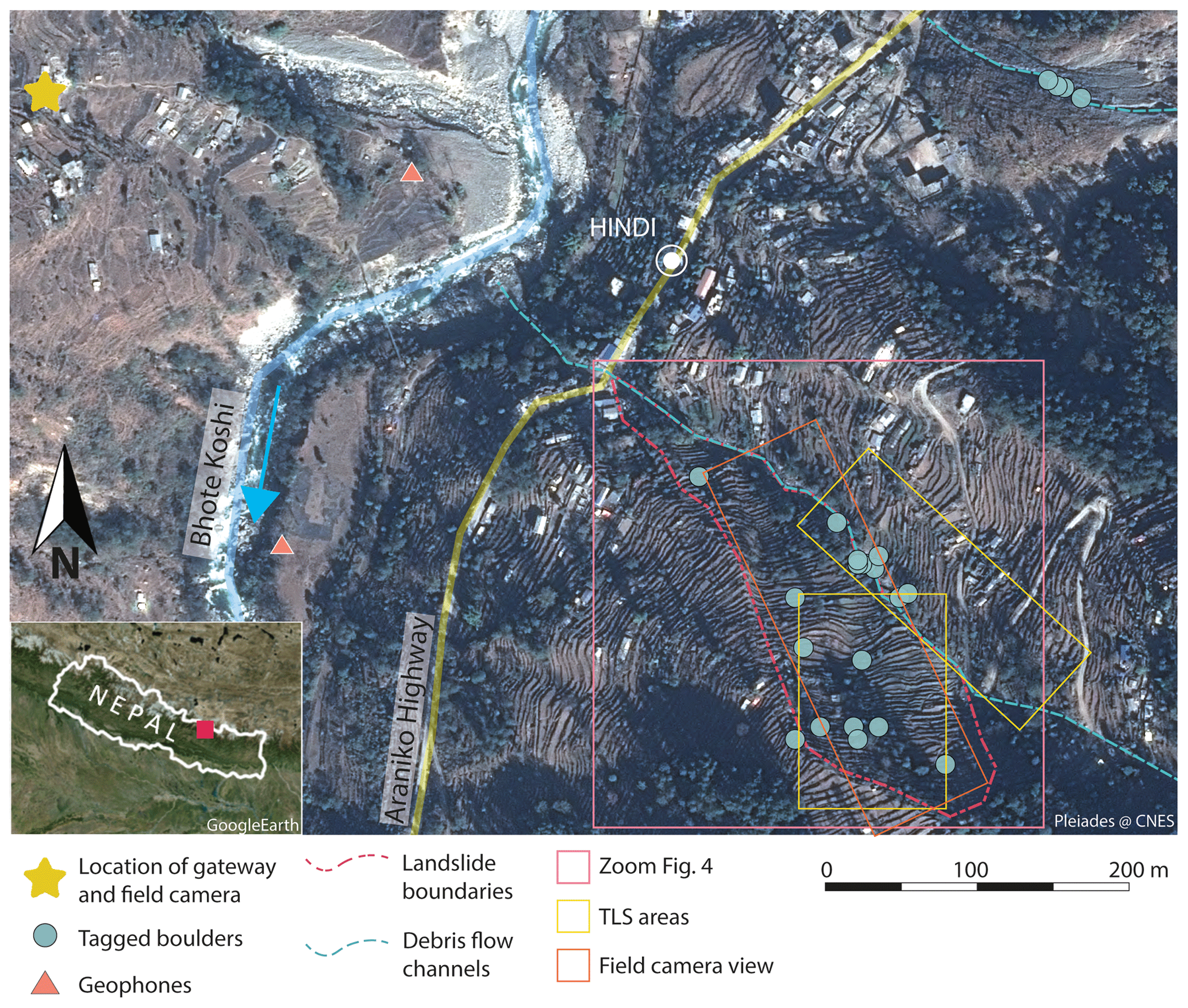
Figure 1Overview of study area and network, including three tagged sites (two debris flow channels and a landslide body). Red box: zoom of two tagged sites. Yellow boxes: terrestrial laser scanner areas. Orange box: field view of the field camera. Image: Pleiades (CEOS Landslides Pilot).
In this study, based in the upper Bhote Koshi catchment (red square in inset in Fig. 1), Nepal, we demonstrate the use of long-range wireless devices to detect hazardous boulder movement and landslide reactivation in real time. We also demonstrate for the first time the use of this technology in the field of geomorphology and in a field set-up to monitor the movement of boulders embedded within a landslide and in two debris flow channels.
2.1 Hazards and their interactions in the area of study
Nepal lies at the heart of the Himalayan arc, and it is one of the most disaster-prone countries in the world. In particular, the extreme topographic gradients, seismicity, and monsoonal climate, coupled with increased population pressure (Whitworth et al., 2020), make Nepal widely and frequently affected by landslides and various types of floods. In 2015 a large number of coseismic landslides were triggered as a consequence of the Gorkha earthquake sequence, in particular in association with the largest M 7.8 Gorkha earthquake (25 April 2015) and M 7.3 Dolakha earthquake (12 May 2015). Several authors mapped coseismic landslides after the events and, although numbers vary greatly (a few thousand to a few tens of thousands of landslides mapped in different studies), the impact of these hazards has been unanimously recognised as very significant (Reynolds, 2018b, c; Roback et al., 2018; Martha et al., 2017; Kargel et al., 2016). The Bhote Koshi catchment, northeast of Kathmandu (red square in inset in Fig. 1), was also identified as one of the most affected areas, showing the greatest density of landslides (Roback et al., 2018; Guo et al., 2017; Tanoli et al., 2017; Kargel et al., 2016; Collins and Jibson, 2015). The areal distribution of landslides away from the main shock epicentre appears to have been controlled by a combination of peak ground acceleration, slope, and fault rupture propagation (Roback et al., 2018; Martha et al., 2017; Regmi et al., 2016). Some authors pointed out that many coseismic landslides occurred at high elevations (e.g. Tanoli et al., 2017), and it was observed that after the earthquake, a large number of landslides remained disconnected from the channels, with significant amounts of material stored on the hillslopes (Cook et al., 2016; Collins and Jibson, 2015), including boulders that are still visible today on valley flanks. During the 2015 monsoon, new landslides were triggered along with the expansion of coseismic landslides, but loose material remained stored on the hillslopes by the end of the monsoon (Cook et al., 2016). The sediments produced with coseismic landslides are expected to move from the hillslopes and into the fluvial system over several years after the earthquake (Collins and Jibson, 2015, and references therein).
The Bhote Koshi is also highly prone to glacial lake outburst floods (GLOFs), with six events reported since 1935 (Khanal et al., 2015). Different authors have mapped glacial lakes within the Bhote Koshi catchment in recent years, with the total number ranging between 74 and 122 (Khanal et al., 2015; Liu et al., 2020), making glacial lake density in this catchment 4 times higher than that of the central Himalaya (Liu et al., 2020). All available studies are in agreement regarding the recent increase in the total area of glacial lakes in the region in relation to increasing temperatures and glacial retreat (Liu et al., 2020), with some authors suggesting that this increase amounts to 47 % and that some lakes doubled in size between 1981 and 2001 (Khanal et al., 2015). Some of these lakes have the potential to drain catastrophically, with some authors indicating that this risk may increase in the future as glacial lakes increase in number and volume. Floods originating from the outburst of glacial lakes can have short-lived discharges that are several orders of magnitude higher than background discharges in receiving rivers (Cook et al., 2018) and can have impacts for many tens of kilometres downstream (Richardson and Reynolds, 2000; Huber et al., 2020; Liu et al., 2020; Khanal et al., 2015). The latest one in the Bhote Koshi catchment occurred in July 2016, likely originating from a rain-induced debris flow into Gongbatongshacuo Lake, a moraine-dammed lake in Tibet (Autonomous Region of China) (Cook et al., 2018; Reynolds, 2018a) that drained catastrophically, impacting infrastructure and properties up to 40 km downstream. Boulders up to 8 m long, weighing in excess of 150 t, jammed the sluice gates of the Bhote Koshi hydropower project, diverting the debris-charged flash flood through, totally destroying the desilting basin, and inducing substantial damage to the site (Reynolds, 2018b). During the remedial works for the reconstruction of the headworks infrastructure, a boulder with a 17 m diameter (approximately 4500 t) was uncovered adjacent to the upstream wall of the headworks dam. This complex event has highlighted the need for improved ways of understanding the interactions of cascading hydro-geomorphic processes and improved measures aimed at increasing resilience (Reynolds, 2018a, c). The availability of loose material on hillslopes, the monsoonal climate, and the GLOF hazard in the area enhance the possibility of material containing large grain sizes reaching the river network via hillslope movements and eventually being remobilised by exceptionally large floods. Huber et al. (2020) highlight the fact that very large boulders (around 10 m in diameter) present today in the Bhote Koshi river have likely been transported by large GLOF events, supporting the idea that it is unlikely that monsoon-generated floods may have the energy threshold required to remobilise very large grain sizes (Cook et al., 2018).
Landslides and debris flows can also occur as a consequence of heavy and persistent rainfall during the monsoon. Every year the area receives up to 4100 mm of rainfall between June and September (Tanoli et al., 2017). Active monsoons can trigger or reactivate landslides; an example is the Jure landslide (roughly 15 km southwest of our study sites) that occurred in August 2014 (Acharya et al., 2016). Moreover, intense monsoon rainfall events can trigger debris flows in low-order stream channels within the region (Roback et al., 2018), thus allowing for movement of some smaller boulders (> 0.25 m diameter) and allowing hillslope–channel coupling.
2.2 Geologic and tectonic setting
Our study sites lie within the Main Central Thrust (MCT) zone (Rai et al., 2017), where the rocks of the Higher Himalaya Sequence (HHS) are thrusted over rocks of the Lesser Himalaya Sequence (LHS). The MCT is one of the main faults that accommodate the subduction of the Indian subcontinent under the Eurasian Plate. The MCT has been mapped at the top and bottom of the roughly 350 m thick Hadi Khola Schist that is sandwiched between the Dhad Khola Gneiss above and the Robang Phyllite below at Tatopani, some 5 km upstream of the study site (DMG, 2005, 2006; Rai, 2011; Reynolds, 2018c). The study site lies entirely within the Benighat Slate, which comprises predominantly black schist, phyllite, quartzite, and carbonate rocks (DMG, 2005, 2006; Rai, 2011). The rocks belonging to the HHS are composed of crystalline amphibolite- to granulite-facies metamorphic rocks, mainly ortho- and paragneisses, quartzite, and schists. The LHS rocks present lower-grade metamorphism, increasing towards the MCT, and are largely comprised of phyllites, schists, metasandstones, and quartzites (Basnet and Panthi, 2019; Martha et al., 2017; Rai et al., 2017; Upreti, 1999; Gansser, 1964).
2.3 Economic assets in the study area – increased vulnerability
Our study sites are located along the Araniko highway, a major route that connects Kathmandu to Kodari and then links Nepal to China. This main road was significantly affected by earthquake-induced landslides in 2015, but it is also subjected to landslides every year during the monsoon season (e.g. Whitworth et al., 2020). The area is of strategic importance for Nepal due to the high concentration of hydropower projects either already in operation or under construction (Khanal et al., 2015). Moreover, the Araniko highway is a key trade and transport link (Liu et al., 2020) and one of the two routes between China and Nepal. Khanal et al. (2015) indicate that international trade and tourism between Nepal and China have been growing rapidly since the opening of the Araniko highway and that this route is economically important; the records of the customs office in Nepal show a value of USD 135.9 million in imports and USD 4.1 million in exports in 2011–2012, with both governments benefiting from the revenue.
2.4 Selected sites
The study site is located at the northern edge of an inferred deep-seated gravitational slope deformation around 1.5 km wide that stretches from Hindi in the north to just upstream of Chakhu to the south (Reynolds, 2018c). A secondary landslide body on the northwest-facing valley flank directly impinging the settlement of Hindi and two debris flow channels were chosen as tagging sites (Fig. 1). The most active debris flow channel of the two marks the northeastern boundary of the landslide, whilst the other channel, which appears to be less active, is located 360 m to the northeast directly upstream of the densest part of the settlement of Hindi. Both channels intersect the Araniko highway and cross the settlement before merging with the Bhote Koshi. The landslide is a soil slide covering an area of approximately 0.03 km2. Colluvium material likely deposited from previous landslides is visible at the head scarp and in the terraces along the southwestern flank, with the presence of large boulders of diameter > 2 m. Large boulders are also observed scattered over the landslide body. The scarp suggests a depth of the landslide of at least 2 m, and large, fresh cracks were observed in the crown area in October 2019, indicating activity during the previous monsoon season.
3.1 Network set-up and components
A total of 23 long-range wireless smart sensors were used as nodes in the system. They comply with the LoRaWAN® (Long-Range Wide-Area Network) specification, are provided with external GPS and long-range antennae, and measure 23 mm by 13 mm (Fig. 2b),. The sensors are equipped with an accelerometer configured to sample at 2 Hz, and a GPS module. In the absence of movement, the devices are programmed to record and transmit one single location (GPS data only) per day at a fixed time. When movement is detected by the accelerometer so that tilt or acceleration exceeds defined thresholds, collection of GPS and accelerometer data is activated. Different thresholds can be applied for a detected angular variation in degrees or for a linear acceleration in g−3. The values assigned for this study can be found in Sect. 3.3. The sensors, which were developed by Movetech Telemetry and Miromico, transmit the acquired data to a LoRaWAN® gateway on the 868 MHz band wirelessly and in real time. A Multitech IP67 LoRaWAN® gateway sends the payloads received from the sensors to a Loriot LoRaWAN® network server through the local GSM network using an agnostic SIM card (Fig. 2a–d). The packages are then sent from Loriot to the Movetech Telemetry server and are decoded, providing the raw information collected by the nodes.
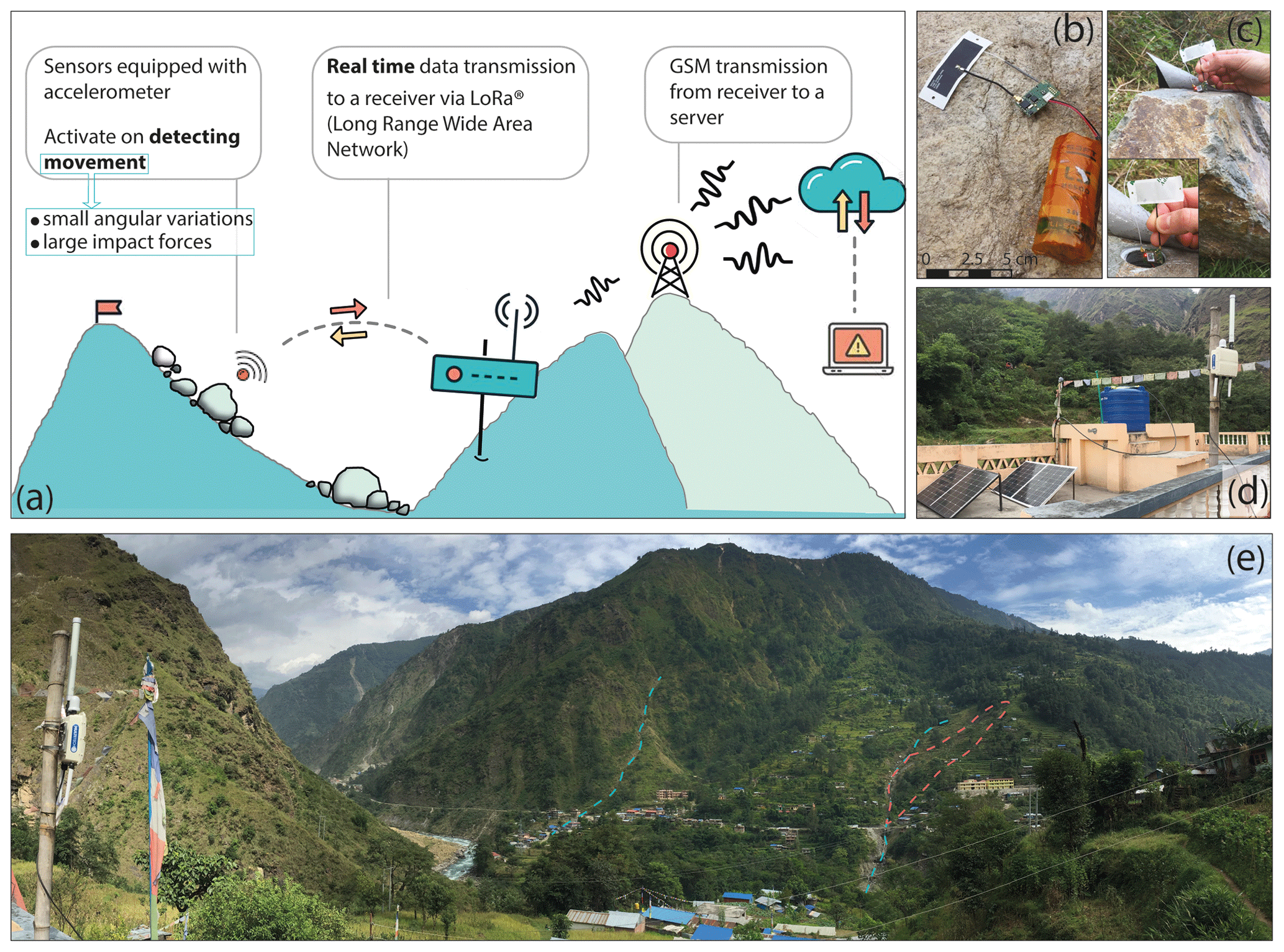
Figure 2(a) Sketch of the network, its components, and communication methods. (b–c) Sensor and tagging of a boulder. (d) Gateway set-up. (e) Overview of the tagging sites from the gateway. The gateway is visible in the far left of the image. Blue dashed lines mark the debris flow channels, and red dashed lines mark the boundaries of the landslide.
Each sensor was fitted with one (Fig. 2b) or two lithium C-cell batteries connected in parallel. A total of 23 boulders were individually tagged by embedding the sensors in a hole drilled in the rock (Fig. 2c). Each boulder was drilled with a 35 mm core drill for a length of about 15 cm. The depth of the hole allowed for the emplacement of the C-cell batteries and the sensor. After placement, each hole was filled with epoxy resin, sealing the cavity and thus protecting the device from tampering and from the elements (water and humidity), whilst allowing for unaffected connectivity to the gateway via LoRaWAN®. To ease the drilling process but also to allow the epoxy to stay in the cavity before being completely cured, the holes were drilled at an almost vertical angle (with respect to the global inertial frame), so roughly from the top down. This allowed for the emplacement of the devices flat against the battery inside the cavity, with the z axis nearly horizontal (global inertial frame), where x and y are oriented as the two longest sides of the device. There is some variability around the deviation from the global horizontal orientation of the z axes of all our devices, but in general terms the position of the device would follow such a set-up. The orientation of the z axis with respect to the cardinal points was not recorded.
The position of the gateway, located in the opposite side of the valley at a distance of about 700 m from the furthest sensor, at 1330 m a.s.l. and roughly 60 m above the valley bottom was chosen to be within reach of the GSM network and have a direct line of sight with the sensors (Figs. 1 and 2e). Due to an unreliable main power supply, a four-panel solar system was developed for this purpose. The initial set-up did not allow for continuous power to the gateway and led to instability in the system, with frequent offline times during the 2019 monsoon season. However, the system has been improved and it will guarantee continuous power to the gateway for successive acquisition seasons. The panels currently charge two 12 V, 110 AH batteries that then provide continuous power to the gateway through a POE (power over Ethernet) supply. The solar system is composed of parts that can be sourced locally at a relatively low cost and that can be transported to sites without road access, such as the site chosen in this study. The nature of the local GSM network, relying on one individual antenna in the area at the time of this study, also led to frequent GSM connection failures, which prevented the gateway from communicating with the server. The devices deployed in the 2019 season were programmed not to store the data but to send them immediately, causing the data transmitted during gateway offline time to be lost.
3.2 Choice of tracked boulders
The tagging sites were selected with the aim of covering different geomorphological settings whilst retaining visibility to the gateway. The boulders identified for tagging are spread over three sites, two debris flow channels, and a landslide body (Fig. 1). The boulders cover a range of sizes and geologies, though the geology in this context is not expected to play a significant role in affecting the connectivity of the network. The smallest boulders tagged have b axes of 0.3 m, whilst the largest boulder has a b axis of 3.3 m (Fig. S1 in the Supplement). The selected boulders are characterised by differences in their position at their location. Boulder location and embedment influenced the choice of the accelerometer settings used, as explained in the section below. They can be subdivided into three categories: in channel (IC), partly embedded (PE), and fully embedded (FE) either within the landslide body or in the channel banks (Figs. 3 and S2). Boulders in the channel are expected to move freely in the case of a large event and to be potentially subjected to collisions. Such events could be debris flows with sufficient intensity to impart forces high enough to cause the boulders to move downslope within the flow. Fully embedded boulders are not expected to move independently of the surrounding soil mass; as such, they can only move as a whole with the material on channel banks or with the landslide body if these were to undergo sliding episodes and reactivation (see example schematics in Fig. 5a, b). For these boulders, generally only the top part is visible, whilst the bottom is fully surrounded by soil. On the other hand, partly embedded boulders found at the head scarp, along the southwestern flank of the landslide, or in the channel banks can either move as a whole with the surrounding material or become dislodged and begin to move freely on the surface. The second scenario is related to the little amount of soil covering the bottom part, particularly in the downslope direction, and this scenario would occur if the soil were to be eroded during intense rainfall events.
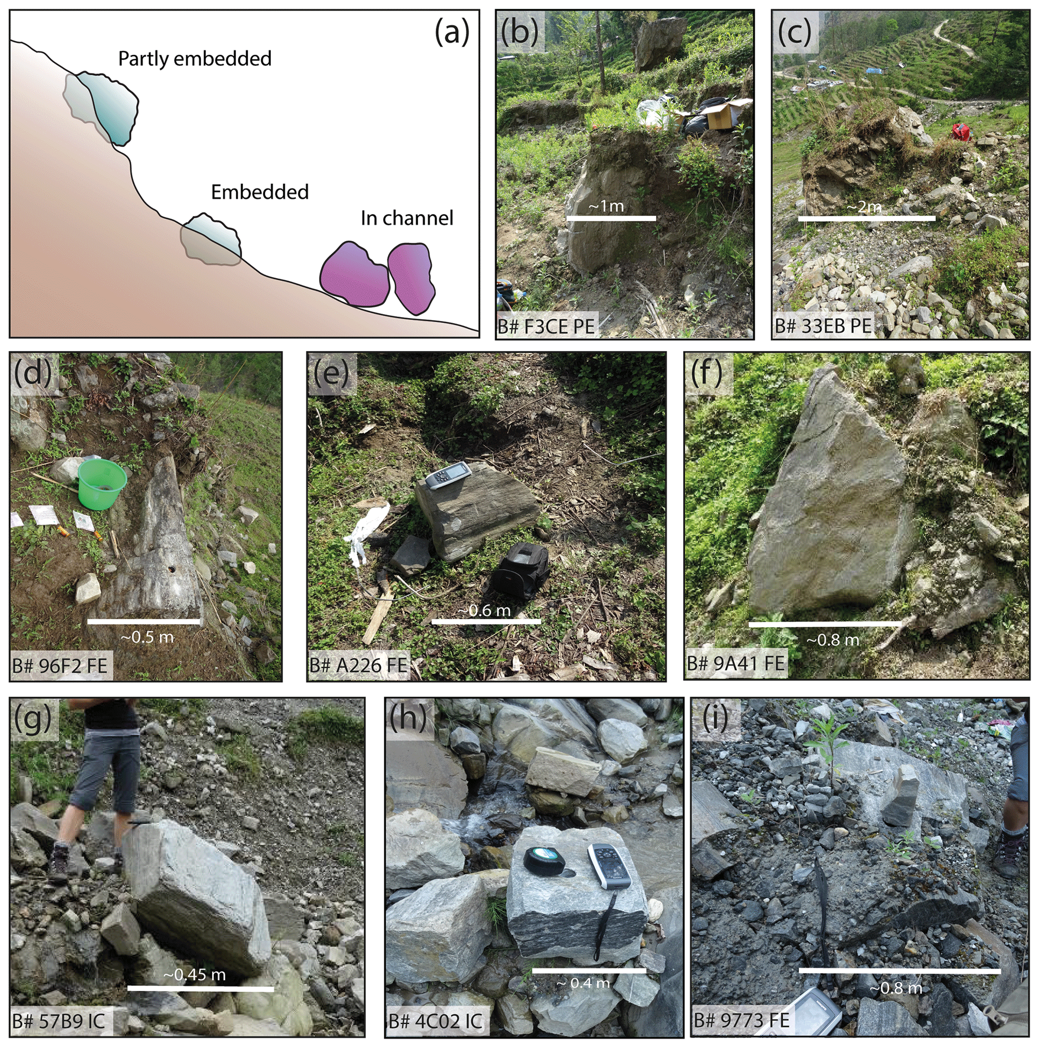
Figure 3(a) Sketch of boulder position types. (b–c) Examples of partly embedded (PE) boulders within the landslide body. (d–f) Examples of fully embedded (FE) boulders within the landslide body. (g–h) Examples of boulders inside the main channel (IC). (i) Example of a fully embedded (FE) boulder within the channel bank.
3.3 Sensor settings
The sensors were programmed to send a routine message every 24 h, in which only the GPS position is sent. Between regular fixes the sensors sleep and do not send any data unless movement occurs, as explained in the following. As mentioned in Sect. 3.1, the sensors can also acquire and send data in association with an accelerometer event for which activation thresholds can be set for impact forces and for angular variations. The sensors can be programmed following two main modes: (1) the accelerometer data are averaged over a window of time (over a number of recordings), and we call this mode average settings (AVG in Fig. S2). (2) The absolute value of the maximum acceleration occurring in a time interval can be recorded, and we call this mode maximum settings (MAX in Fig. S2). In the first case, the values of the three axes are normalised to g force (where 1 = 1 g), and the measurements essentially represent the static angle of tilt or inclination; thus, the projection of the acceleration of gravity, g, on the three axes ranges between 0 (for an axis oriented horizontally with respect to the global inertial frame) and ±1 (for an axis oriented vertically with respect to the global inertial frame). In the second case, the absolute maximum value can be recorded; this can exceed 1 g and can be set as high as 2, 4, 8, or 16 g. The measurement resolution changes according to the chosen detectable maximum so that a scale capped at 2 g has a resolution of 0.016 g, whilst a scale capped at 16 g has a resolution of 0.184 g (Fig. S3).
When considering only an individual axis, the variation between two static accelerometer measurements would correspond to an angular change, as shown in Eq. (1):
where γ is the angular variation on a given axis and m is the difference between normalised successive accelerometer values recorded on the same axis in g. Eq. (1) describes the relationship between accelerometer output on a given axis and its tilt: for trigonometry, the projection of the gravity vector on an axis produces an acceleration that is equal to the sine of the angle between that axis and a plane perpendicular to gravity. According to Eq. (1), if the scale is capped at 2 g, for m=0.016 g the corresponding angular variation is approximately 0.9∘ if the axis is vertical (with respect to global inertial frame) but approximately 5.5∘ if the axis approaches horizontal. Similarly, if the scale is capped at 16 g, a value of m=0.184 g corresponds to an angular variation of about 10∘ when the axis is nearly vertical, but this increases to as high as approximately 21∘ when the axis approaches the horizontal (Fig. S3).
The boulders expected to move as a whole with the soil in which they are embedded, and that are more likely to experience small and gradual angular variations as the surrounding material gently slides, were programmed with the average settings. We chose to cap accelerometer data for average settings at 2 g (highest resolution), as high-impact forces were not expected, and we assigned thresholds for activation to accelerometer events of approximately 0.4 g and 5∘ for impact forces and angular changes, respectively. The sensors in the two debris flow channels and some of those only partly embedded within the landslide were programmed to record high-impact forces using the maximum settings (Fig. S2). In this case, the scale was capped at the maximum detectable force of 16 g (lowest resolution), and the impact and angular thresholds were set at approximately 4 g and 5∘, respectively. This angular threshold yielded noisier data with respect to the sensors programmed with the average setting type because of the direct consequence of a drastic reduction in measurement resolution in the sensors programmed with the maximum setting type (Fig. S3), for which the scale was capped at 16 g. Natural measurement variability and errors associated with the sensors led to spurious data, given the relatively small angular threshold assigned for the highest detectable maximum of 16 g. In other words, given that the step of accelerometer measurement is as high as 0.184 g, a spurious angular variation of more than 5∘ is often detected even when the boulder is stable due to intrinsic measurement variability (up to 2 bits). Due to the fact that an angular threshold lower than the scale resolution was imposed, we observed many extra acquisitions triggered by small variability in accelerometer measurements around a stable value rather than by true movement.
In order to reduce the noise in the data due to these fluctuations, a three-stage smoothing is applied to the raw data. First, a moving window covering five successive data points is used. The median value of the five data points is assigned to all points in the window that lie within ±0.184 g of the data point immediately before the window. If any of the values lie outside the ±0.184 g threshold, then the raw data points are left unchanged. In the second stage, peaks of one data point are removed (i.e. one point above or below two points with the same value); this is because if a high-impact force is imparted to a boulder, the position of the boulder is expected to change. This would mean that a high value would likely be followed by a change in the static angle of tilt of the three axes. Therefore, it is unrealistic to have a peak value followed by a value equal to that observed before the peak, particularly when sampling at 2 Hz. This would imply that a boulder undergoes acceleration in one direction, moves, and comes to a halt in the same orientation as before the movement. In the third and final stage, another moving window of five consecutive data points searches for values that lie within the ±0.184 g threshold with respect to the last point immediately before the window. The same value of the last point before the window is assigned if all points are within the threshold. If any of the points lie outside the ±0.184 g threshold, the values are left unchanged.
After smoothing, time series of actual accelerometer values were referred to the same zero only for visualisation purposes, without further manipulation. The accelerometer x, y, and z values were recalculated simply as
for i > 1, where xt is the transformed, plotted value and xi all measurements after the first. This allows the graphs shown in Figs. 5 and 6 to be analysed more easily, preventing the y-axis scale from being stretched between −1000 and 1000 mg.
Finally, schematic visualisations of a sample model boulder were produced, calculating pitch and roll angle changes from the actual data (Supplement Sect. S1), to indicate the amount of rotation boulders in the channel underwent (Fig. 6b, d, f). The boulders in the 3D visualisations are, however, extrapolated from the context of the channel in which they were at the moment of tagging because it is not possible to calculate the yaw angle (i.e. the angular variation around the global vertical). The purpose of the visualisations is just to give a sense of the change in orientation obtained by the boulders between successive accelerometer measurements (Fig. 6a, c, e), and not that of offering a full 3D representation of boulder movement.
The sensors are equipped with a GPS module, which is currently also used to retrieve the date and time of the data acquisition, whilst the data transmission has another time stamp related to the arrival of the data string to the server. The accelerometer readout in the current version of the software is tied to a GPS acquisition; this means that although the accelerometer is activated as soon as movement is detected, the recording of the acquisition is obtained only when the GPS has successfully retrieved the position. An acquisition of accelerometer data with no GPS position can be obtained and transmitted (in which case it would only be associated with a server time stamp indicating time of arrival at the server), but only after the GPS has attempted to retrieve the position and failed. The time-out for the GPS search has been set to 120 s. This is because, due to the local topographic setting and the high valley flanks, the availability of enough satellites at any given time may be low. A major drawback during the 2019 acquisition campaign was that during the GPS search time, no accelerometer acquisition could be recorded and transmitted in the current firmware version of the devices. This means that if boulder movement unfolds over a few seconds, the likelihood is that the accelerometer recording will only occur towards the end of the movement or after it has stopped completely, allowing only the retrieval of snapshots of information on two successive static acquisitions within seconds (near-real time) of the movement starting. Development has already been made to the firmware to separate the accelerometer acquisition from the GPS for future acquisition seasons and increase the velocity of the accelerometer response to a trigger.
3.4 Validation data
A Bushnell NatureView HD camera was installed at the gateway location. The camera was set to acquire an image every 30 min, and the field of view included the landslide and the southwestern debris flow channel to around 35 m below the Araniko highway. Given the rugged terrain and the line of sight, the visibility in the area around the southwestern flank of the landslide is limited and the observation is best for the lower part of the slope. Moreover, the plane of the landslide is at a relatively low angle with the line of sight of the camera. Image cuts were performed for analysis over the visible parts of the southern channel and of the landslide (Fig. 1). Pixels visually recognisable in all image frames were manually selected. These correspond to individual trees or boulders and were identified in successive frames. This allowed for a rough estimate (with an accuracy of about 0.2 m) of the displacements of these features in the image plane through the available image sequence.
Moreover, the landslide body and the southwestern channel (Fig. 1) were scanned with a Faro Focus 3D X330 terrestrial laser scanner (TLS) in two successive campaigns in April and in October 2019. Each site was scanned from two scan locations, and the point clouds were aligned by matching stable areas using the multi-station adjustment algorithm in Riegl RiSCAN Pro (v. 2.3.1). The data were analysed to obtain ground displacements during the monsoon season and processed using the point-to-point cloud comparison method M3C2 in CloudCompare (Lague et al., 2013). The field camera and TLS data were used to identify days characterised by sliding of the landslide body, sliding of the channel banks, boulder movements, and areas that underwent significant changes of the ground surface. These data are used in a qualitative way for comparison with and validation of the accelerometer data obtained with the wireless devices, and, despite the qualitative approach, these data provided a quite detailed overview of the days on which movement occurred. Two Pe6B three-component geophones recording at 200 Hz were installed on fluvial terraces below the study site to monitor debris flow activity in the debris flow channels (Burtin et al., 2009).
We observed that during the 2019 monsoon season, there were important sliding episodes of the main landslide body (see Sect. 4.1), which caused small and gradual tilt of the tagged boulders embedded within it. Moreover, although there is no evidence of large debris flows in either of the channels tagged (for example, in the seismometer records), some boulders within the southern channel bounding the landslide show data that could indicate rapid movement. Of the 23 boulders tagged, 9 show accelerometer time series that are compatible with downslope movement (yellow to red symbols in Fig. 4). Of these, six lie within the landslide body and were programmed with the average settings in order to detect small angular changes (Fig. 5). The remaining three were located within the southern debris flow channel and were programmed with the maximum settings to capture large (> 1 g) impacts (Fig. 6).

Figure 4Zoom of two tagged sites. The sizes are scaled according to the b axis of the boulders (an example of scales is given for boulders without movement in the legend, but it applies to all boulders). White squares are boulders that did not move or for which movement was not recorded. Green circles are boulders in the debris flow channel. Yellow to red symbols are boulders within the landslide body. Hatched areas are zones with observed movement through images (L: lower, M: mid-slope, U: upper) and terrestrial laser scanning. Image: Pleiades (CEOS Landslides Pilot).
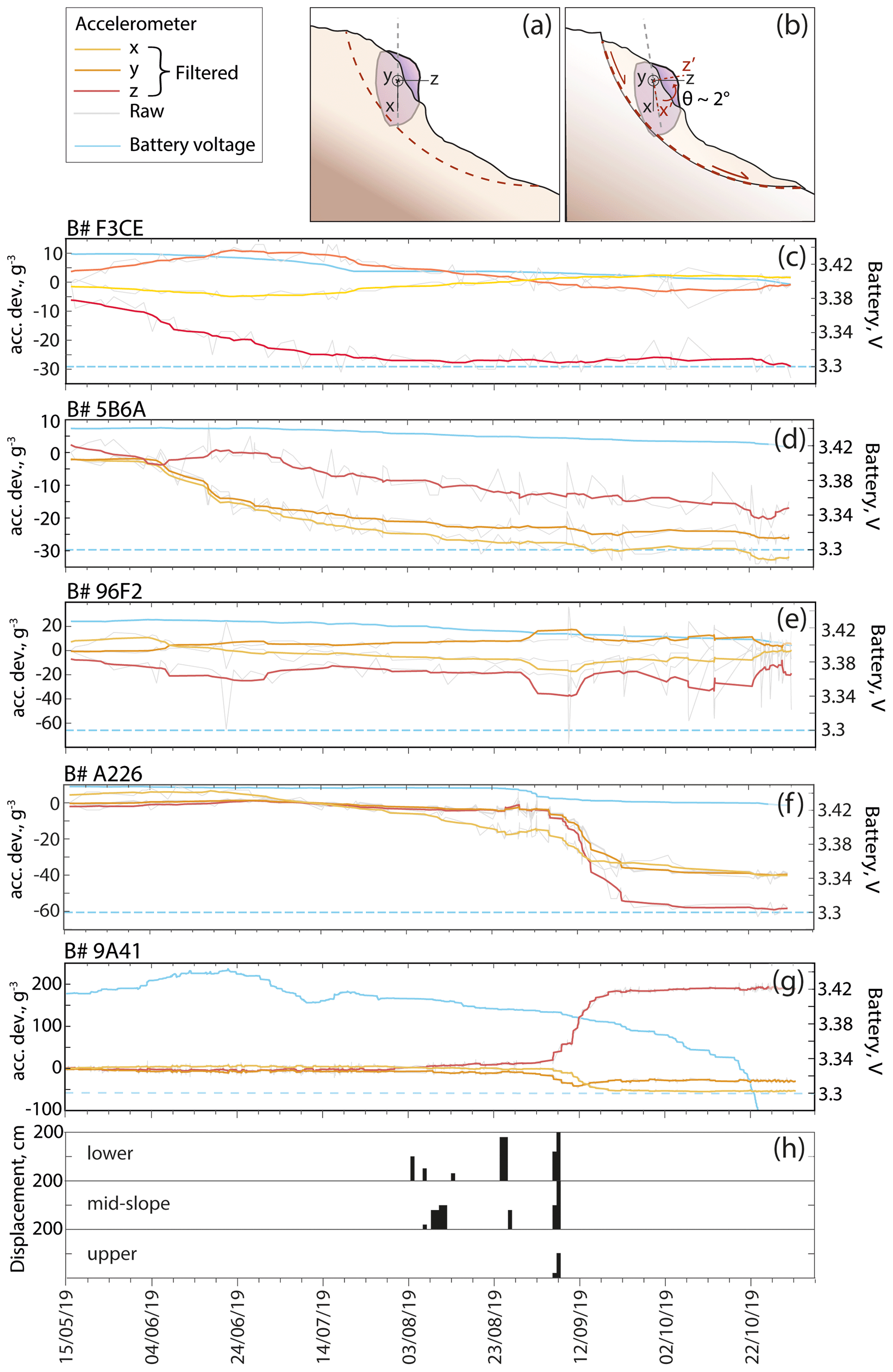
Figure 5(a–b) Sketch of the possible type of movement experienced by embedded and partly embedded boulders. Note that this is only a schematic to indicate a movement that occurs in accordance with the landslide body and does not necessarily represent real movement of the boulders monitored in this study. (c–g) Real accelerometer data (raw and smoothed) showing deviation from the initial position for each axis for boulders within the landslide body through the monsoon season. The yellow, orange, and red curves in the line plots represent the smoothed data from the accelerometer x, y, and z axes, respectively, and the grey curves represent the raw data for each axis. The blue curve shows the battery voltage, and the blue horizontal dashed line represents the 3.3 V threshold below which the battery is discharged and faulty behaviour may be expected. (h) Estimated displacements of lower, mid-slope, and upper parts of the slope obtained through field camera images.
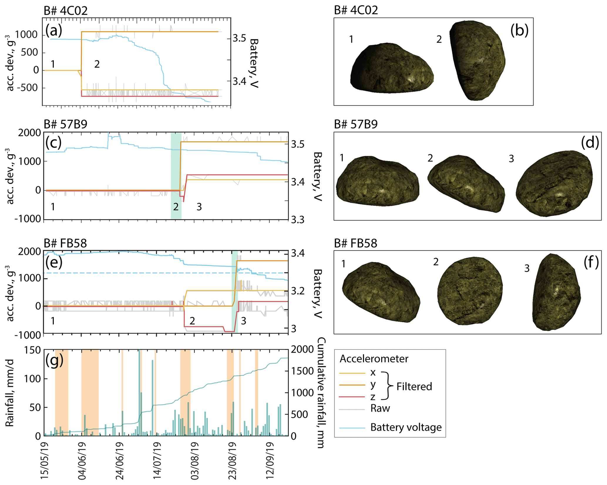
Figure 6(a, c, e) Real accelerometer data (raw and smoothed) showing deviation from the initial position for each axis for boulders in the debris flow channel and its banks through the monsoon season. Light green bars represent uncertainty in the movement timing due to lack of GPS acquisition (i.e. no time recorded) or an offline gateway. (g) Daily and cumulative rainfall data from GPM. Yellow bars represent days on which movements are observed in the channel and/or on its banks in the field camera images. (b, d, f) Model boulder 3D visualisation to represent the change from the initial positions of the boulders and the positions acquired after the recorded movement, only in terms of pitch and roll angles (see Supplement Sect. S1). Note that the boulders are in a space with no coordinates because the visualisations do not indicate the position of each boulder within the channel, but only the pitch and roll angle changes. Numbers of positions are marked in the accelerometer graphs.
In terms of boulder sizes, boulders that appeared to have moved within the landslide have b axes ranging from 0.4 to 2.75 m, whilst those that moved in the southern channel have b axes between 0.4 and 0.5 m (Fig. S1), thus covering a much smaller range.
The four boulders within the landslide that do not show evidence of movement (white circles in Fig. 4) were fitted with sensors programmed with the maximum settings (Fig. S2) due to the fact that they are partly embedded in the landslide and had potential to become detached from the landslide body. Thus, given the lower accuracy and coarser scale, they could not have detected small, gradual movements even if they had been subjected to them.
4.1 Slow movements within the landslide body
The movement recorded by boulders embedded within the landslide body is consistent with slow, gradual tilting that occurred with the sliding of the landslide mass. Small rotational components of the displacement vector that can either be related to the whole mass or, most likely, to different sectors of the landslide induce small angular variations to the boulders embedded within the soil at the surface. Figure 5 shows the accelerometer data for fully and partly embedded boulders programmed with the average settings. The graphs in Fig. 5c–g show the values recorded by the accelerometers in the x, y, and z axes through the observation window. Time is shown on the x axis from 15 May to 31 October 2019, whilst the y axis indicates the value of the projection of g on each accelerometer axis in milligrams (g−3). The grey curves are raw data, and the yellow, orange, and red curves are the data after noise was removed. The data are actual data recorded by the accelerometers, referred to a common zero for visualisation purposes, as explained in Sect. 3.3 (hence, all raw data curves begin at zero and the smoothed curves around zero due to the smoothing). A sketch of the possible type of movement related to gentle tilting of the boulder within the soil mass is shown in Fig. 5a and b and does not represent any true movement of any of the tagged boulders. The data show that all sensors that detected movement were appropriately charged throughout the season (blue curves in graphs). The variations of the accelerometer axis values from the initial value range from 10 mg to 200 mg in the different sensors. For an individual axis, the variation in the values would correspond to an angular change as shown in Eq. (1). Thus, for m=10 mg, γ≅0.6∘ and γ≅8∘ for a nearly horizontal and nearly vertical axis (with respect to the global inertial frame), respectively, and for m = 200 mg, γ≅12∘ and γ≅37∘ in the horizontal and vertical cases. In all boulders the rotation is oblique with respect to all axes and does not occur around any of them.
The images acquired by the time-lapse camera (see the Video supplement) indicate that the landslide moved slowly at the beginning of the rainy season and then accelerated later in the season, most likely in relation to an increase in the pore water pressure within the soil. This temporal evolution is also observed in our accelerometer data. Moreover, it is likely that the landslide is divided into sectors with different activity levels and different responses to rainfall through time (e.g. Bonzanigo, 2021). In particular, Figs. 4 and 5 show that the movements of boulders within the landslide not only differ in the magnitude of the angular variations recorded, which is an order of magnitude higher for B-A226 and B-9A41 in comparison to other boulders, but also in the evolution with time. Three boulders (B-33EB, not shown in Fig. 5; B-F3CE and B-5B6A, the positions of which are also labelled in Fig. S2) already show movements early in the time series during May and June. The other three boulders (B-96F2, B-A226, and B-9A41) show a later onset of the movement between late August and mid-September. The boulders with early movements are located below the main scarp (B-F3CE) and in the middle part of the landslide (B-33EB and B-5B6A) closer to the channel, whilst those that move later are closer to the southwestern flank of the landslide (B-9A41 and B-96F2), thus farther away from the channel and in the lower half of the landslide body (B-A226).
Visual interpretation of the images acquired by the field camera (Sect. 3.4) indicates that significant movements of the landslide body occurred during sliding episodes within the orange hatched area in Fig. 4. The area in which visible changes occurred is about 5000 m2 and corresponds to the lower portion of the landslide. Figure 5h indicates the estimated movement magnitudes in the image plane for the lower, middle, and upper parts of the visible sliding area (indicated by L, M, and U in Fig. 4). Displacements roughly up to 2 m in the image plane are detected in the lower and mid-slope parts of the moving area (Figs. 5h and 7a) between the end of August and the beginning of September, with upper parts showing displacements of around 1 m. The movement observed in the accelerometer data of B-A226 and B-9A41 (Fig. 5f–g) corresponds to the periods in which higher displacement magnitudes are inferred from the images. Figures 4 and Fig. 7b also show that boulders B-5B6A, B-33EB, and B-9A41 are located in areas surrounded by displacements as seen by the TLS data (yellow hatched areas in Fig. 4). Moreover, two boulders within the upper part of the landslide were not found in the field campaign carried out in October 2019 (B-33EB and B-625C), likely due to fresh accumulation of material from the scarp. Indeed, TLS scan data show cumulative displacements of up to 1 m over large areas between April and October 2019 (Fig. 7).
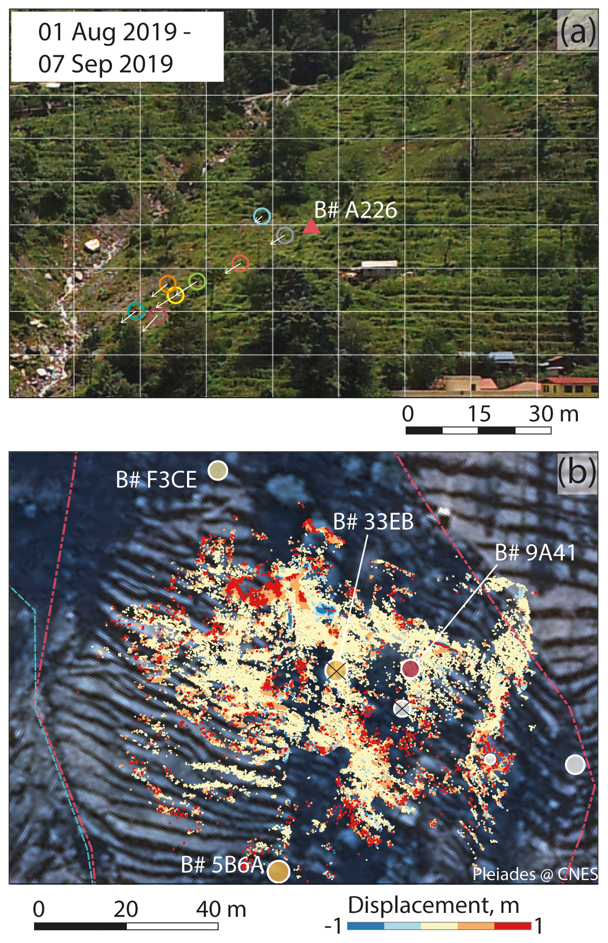
Figure 7Examples of movements in the landslide body between panels (a) and (b). Coloured circles visually represent traceable pixels. Their movement is visible through the superposed grid. The approximate location of B-A226 is shown. (c) Scan data for the upper part of the landslide area show several zones of movement; red represents accumulation and blue erosion. Black crosses represent boulders that were not found after the monsoon season. Image: Pleiades (CEOS Landslides Pilot).
4.2 Rapid orientation changes in boulders in the southern debris flow channel
Figure 6 shows the accelerometer data obtained for boulders located within the southern debris flow channel or on its banks between 15 May and 22 October 2019. The graphs in Fig. 6a, b, and c contain the same accelerometer information as explained in Sect. 4.1. The difference in the scale of the accelerometer output with respect to Fig. 5 is explained by the different settings. These boulders were programmed to retrieve accelerations higher than 1 g (as opposed to normalised values) and forces up to 16 g. The raw data (grey curves) show frequent oscillations, often within ±0.184 g around a value (corresponding to one step in the accelerometer scale, or 1 bit) and occasionally up to ±0.372 g (two steps in the scale, 2 bits), associated with measurement variability and the coarse scale used (see Sect. 3.3).
As an example, in the graph for B-4C02, we observe a change from the initial orientation of the accelerometer within the boulder equivalent to 1000 mg in y and around 700 mg in x and z. This is compatible with a change between the initial orientation 1 and orientation 2 attained by the boulder by 4 June 2019, as visualised in Fig. 6b. The current settings have not captured how the boulder transitioned between position 1 and position 2, likely due to the very short time interval during which the change is expected to have happened. The GPS acquisition is likely to have taken longer than the movement that triggered the recording and delayed the accelerometer acquisition. This applies to the other two boulders shown in Fig. 6. We do not observe forces > 1 g for any of the sensors programmed with the maximum settings, despite the ability of the sensors to detect up to 16 g. This is consistent with a lack of debris flow activity recorded by cameras or seismometers, the more prolonged activity of which would have generated sustained boulder movement, beyond the time needed for GPS acquisition as explained below.
Figure 6g shows rainfall data (daily and cumulative) from GPM IMERG (Bolvin et al., 2015) in green, while the orange bars indicate days on which movement (sliding of the banks and/or individual boulder movement) is observed within the channel in the images acquired by the field camera. Often periods with movement observations occur after days of moderate to intense and/or persistent rainfall. B-4C02 shows movement data recorded by the accelerometer as early as the beginning of June. Even though this is early in the monsoon season, this movement falls within a few days of moderate rainfall at the beginning of June during which movements in the channel are already visible in the camera's images. Similarly, B-57B9 and B-FB58 show movement (i.e. changes in orientation) very close in time to periods for which other movements are visible within the channel in the images. Just as an example of the several boulder movements observed in the channel in the camera images, a boulder movement that occurred roughly 25 m downstream of the tagging area in early June is shown in Fig. 8a–b, where two boulders can clearly be seen to move downslope from the banks towards the middle of the channel by 2–5 m. Figure 8c shows the areas on the northeastern channel bank and the channel bed for which significant changes in the ground surface during the monsoon season are detected with the TLS data. Here, erosion exceeding 1 m is observed in the northeastern bank, and accumulation exceeding 1 m is observed in parts of the channel bed.
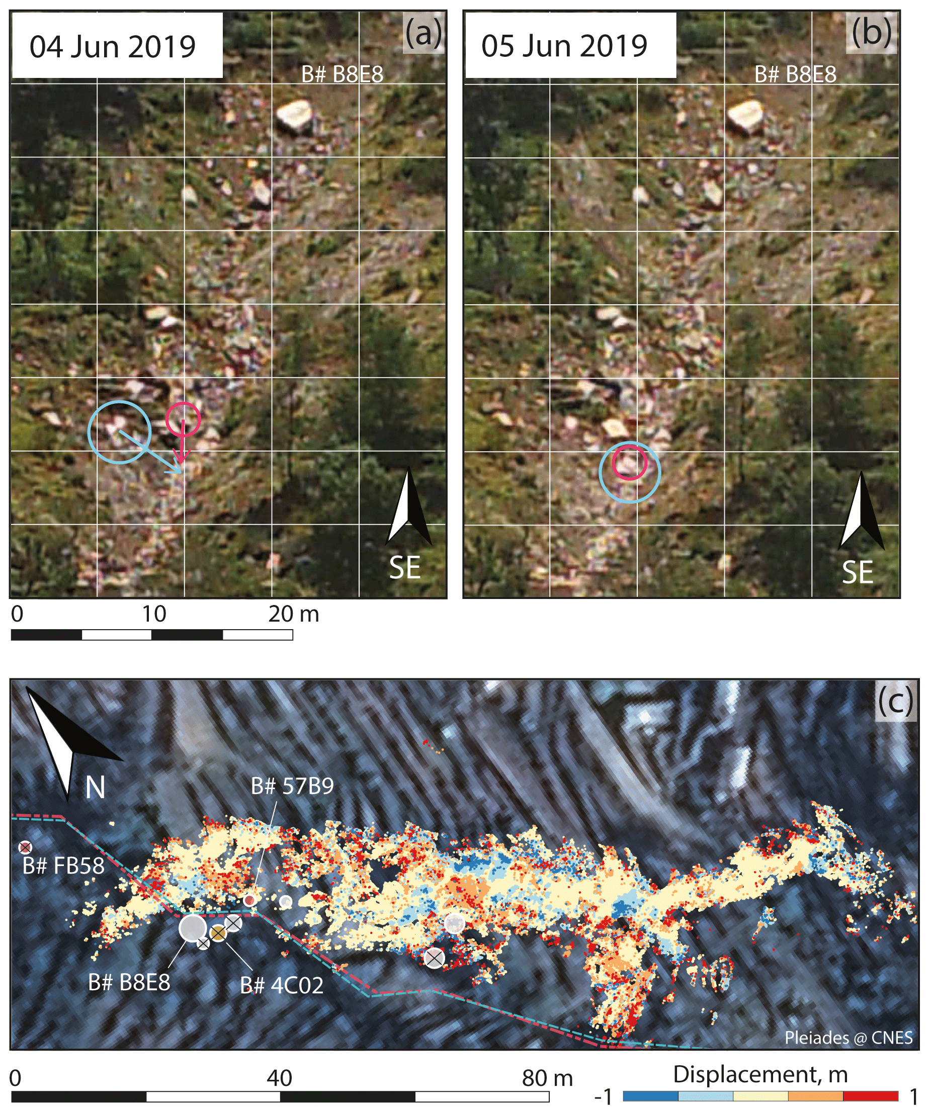
Figure 8Example of movements in the debris flow channel between panels (a) and (b). Example of movements in the channel banks and in the channel between panels (c) and (d). Coloured circles represent traceable pixels. Coloured boxes represent areas in which large changes are observed. (e) Scan data for the channel showing several zones of movement; blue represents a collapse of parts of the orographic right bank, and red represents accumulation areas. Black crosses represent boulders that were not found after the monsoon season. Image: Pleiades (CEOS Landslides Pilot).
The vertical green bars in the graphs for B-57B9 and B-FB58 (Fig. 6c and e) show the uncertainty regarding the timing of the recorded movements. Essentially, each green bar indicates a window of time during which the movement observed may have occurred. The data for each orientation change marked by a green bar may have been transmitted at a different time than the acquisition time, as explained below. An explanation of the different scenarios that are described below is also given in the flowchart in Fig. 9. The orientation change of B-4C02, the second event of B-57B9, and the first event of B-FB58 are characterised by an equal GPS time stamp (time of acquisition) and server time stamp (time of transmission). This indicates that the data transmission occurred within seconds of the data acquisition (real time). B-57B9 shows two changes in orientation between 26 and 30 July 2019. The sensor experienced a gap in the GPS time stamp between 06:15 UTC on 22 July and 06:21 UTC on 28 July, as the GPS failed to obtain a position during this time. Moreover, during this period the gateway temporarily went offline. For these reasons, it impossible to know whether the movement that caused the orientation change shown in the data transmitted on 26 July occurred immediately before transmission or during the window for which the GPS time stamp is not available. The gateway experienced another offline period between 09:36 UTC on 28 July and 03:51 UTC on 30 July, by which time the data show that an orientation change had occurred. Although the acquisitions have both GPS and server time stamps and these are the same (i.e. acquisitions sent in real time), the actual movement may have happened at any time between those two time stamps.

Figure 9Flowchart illustrating the presence of a GPS time stamp (GPS TS) and server time stamp (SV TS) as well as the different scenarios of GPS acquisition and data transmission.
During the period encompassing the two recorded movements (26–30 July), the field camera images indicate overcast, rainy conditions that corresponded to important sliding of the right bank of the channel, offering supporting evidence for movement within the channel. B-FB58 sent data from 15 August 2019 up to 07:17 UTC on 24 August 2019 regularly (based on the server time stamp) but without a GPS time stamp. A small gap follows, due to the gateway being offline from 07:17 UTC on 24 August until 16:00 UTC on 25 August, by which time the change in orientation had occurred and the GPS and server time stamps are the same (data sent in real time). Thus, the second movement of B-FB58 is likely to have occurred between these two times, even if the data acquired after the gateway was online again were sent in real time on 25 August. The camera images show that movements on the right bank of the channel occurred between 22 and 24 August. The scan data also show important displacements in the channel right bank (Fig. 8c). Moreover, five boulders in the channel (or on the bank) were not found in October 2019 at their original location. Two of these are boulders that appear to have moved in the smart sensor data, and the other three may have been covered by deposition of loose material.
No boulder movement was recorded for the northern channel, and field observations in October 2019 revealed no signs of recent activity in the channel, which was completely overgrown with vegetation.
4.3 GPS module limitation
The GPS had an overall poor performance across all the sensors during the data acquisition season. The average success rate of GPS acquisition (the ratio between the number of acquisitions with a GPS time stamp and all acquisitions) for the 23 sensors is around 49 %, with two sensors never acquiring a GPS position throughout the time they were active. Moreover, the standard deviation of positions ranges between 4.3 and 15.8 m in the x and 5.5 and 22.6 m in y after removing outliers. The GPS data acquired are unrealistic not only for the magnitude of the position differences of the same boulder, but also because the direction is often inverted in time, which is not compatible with possible boulder movement. However, the poor performance of the GPS for the purpose of boulder tracking has only a limited impact on the ability to detect movement or orientation changes using the accelerometer, as outlined in the previous sections.
Our data show that 9 out of 23 sensors emplaced in boulders at our tagging sites transmitted data compatible with real boulder movement, indicating the potential of the technology to be used for detecting the onset of boulder movement in real or near-real time. Such onset of movement is observed as both the change in static tilt associated with gradual angular variations and as larger changes in boulder orientation associated with rapid movements. Although describing the full 3D representation of boulder movement is beyond the scope of this paper, this result, based on the first deployment of this network, is very promising for the use of this technology in early warning systems in the future because it shows that the onset of movement can be identified in real time, provided that all components of the network operate correctly.
The movements observed for the boulders scattered on the landslide body and embedded within the material can be described as small angular variations that occurred gradually during the season. Visual recognition of such movements in the field or in the camera images and scan data would be unfeasible for individual boulders because they correspond only to small tilt that is difficult to detect with such methods. However, there are elements that support the fact that the data acquired by the accelerometers are real and caused by gradual tilting. The images acquired by the camera show important sliding of the landslide up to 2 m in August–September (see Sect. 4.1 and Fig. 7a), when the boulders located around the southwestern flank and in the lower part of the landslide show a higher magnitude of the angular variations with respect to other boulders (Fig. 5f, g). The fact that the onset of movement observed in six boulders in the landslide is not random but appears to follow a spatial and temporal pattern also supports the idea of a landslide reactivation that causes smaller movements around the head scarp and nearer the channel to occur earlier. The head scarp activity may not only be related to the movement of the entire mass, but also to small collapses of the colluvium material in the steep exposure. This may have already led to small movements from the onset of the monsoon. Movements in this area are supported by data obtained with the TLS that indicate that displacements in the line of sight of up to 1 m occurred at or just below the head scarp during the season (Fig. 7b). Moreover, two boulders in this area were not found in October 2019, most likely because they have been covered by collapses of loose material from the head scarp. The area near the northeastern flank may have experienced an increase in pore pressures due to earlier saturation of the soil here than in the area at the opposite flank, also related to a more rapid increase in the groundwater table nearer the channel driven by topography. We also observe that the magnitude of movements of boulders closer to the southwestern flank and in the lower slope is higher than elsewhere; this is well supported by observations obtained through the field camera.
Four partly embedded boulders in the landslide (Fig. S2) were programmed with the maximum settings and showed no movement (Fig. 4). The reason to choose this setting type for these boulders is that the nature of their position (PE) may have led to larger and faster downslope movements if they had become dislodged. Given the lower resolution of the data obtainable from the maximum settings, it is possible that nothing would have been observed for these boulders even if they had moved consistently with the landslide body and experienced slow and gradual tilting of a few degrees. In other words, it is possible that such boulders also moved but that the nature of the movements may have been too subtle to be captured with the settings applied. It is also possible that these boulders found themselves outside the active sectors of the landslide, although this seems less likely given the observations obtained in the field and also from camera images and scan data. Although camera images, scan data, and accelerometer data are characterised by different time resolutions, the movements observed in both the landslide and channel in the images and the amount of erosion and deposition observed in the scan data indicate that the boulders tagged were likely involved in such movements, and thus there is increased confidence in the fact that the accelerometer data indeed indicate real movement of the boulders.
Another element that supports the fact that the recorded accelerometer data are associated with real boulder movement is related to boulder size. Figure S1 shows boulder sizes for boulders with and without movement in the three different tagging sites. For boulders within the landslide body, a size control on movement was not anticipated. This is because boulders were expected to move as a whole with the landslide mass, and thus their potential to be transported would be independent from their size. On the contrary, in the channel, and particularly for boulders lying in the channel bed, a size control on movement is expected because the size of boulders that could be mobilised by a flow depends on the flow intensity (Clarke, 1996). Therefore, a flow with low intensity could not be expected to mobilise the largest boulders tagged. The observations indicate that boulders that show movements in the landslide are characterised by a much higher range of b axes than those in the channel (Fig. S1).
For boulders programmed with the maximum settings, we observed noisier accelerometer data than for those programmed with the average settings. What controls this behaviour is not the fact that the sensors were programmed to detect the maximum force or the static tilt, respectively, but rather the scale that was chosen and associated with the two setting types combined with the choice of the angular threshold to trigger acquisitions. As mentioned before, 16 and 2 g were chosen as values to cap the scale in the maximum and average settings, respectively.
When a sensor is programmed to be capable of capturing forces impacting a boulder as high as 16 g, the resolution currently available for the accelerometer's reading is 0.184 g. Although this is a relatively small value with respect to 16 g, it corresponds to an angular variation of 10.7∘. Moreover, we observe that measurement variability is often 1 bit but occasionally 2 bits, the latter corresponding to 0.372 g and an angular variation of 21.8∘. As the sensors can be activated on both an angular threshold and an impact threshold detected on any of the axes, care must be taken when selecting the angular threshold in relation to the achievable accuracy. An angular threshold of 5∘ at this resolution is below the measurement error and can trigger a large amount of spurious data strings. This has the negative effect of diluting the signal with noise and, crucially, reducing battery lifetime. The downside of programming sensors with the settings for high-impact recording is that small angular variations cannot be detected. Future improvements of the accelerometer accuracy, resulting, for example, from the activation of the nine-axis IMU present in the hardware of the devices, could reduce this problem.
Although the GPS module is expected to produce readings with a positional error of less than 2 m in normal conditions, we observed a significant increase in the standard deviation of the measurements in northing and easting. This could be caused by three effects: (1) the narrow valley drastically reduces the visibility time of any passing satellites and thus the chances that a suitable number of satellites will be available to each sensor for calculating the position; (2) the GPS is activated relatively rarely, and this may reduce accuracy (and thus in time precision) of the obtained positions; (3) the rock in which the sensors are embedded appears to deteriorate the signal. Experiments carried out at the sites have shown that even sensors placed outside a boulder, held in the open air and away from obstacles, needed several minutes to get a GPS position. Moreover, experiments carried out in the UK, at an open site, have shown that the same sensors at the same site retrieved a position within a radius of about 50 m when placed inside a boulder and within a radius of about 2 m when held in the open air. The acquisition of a GPS position is also what causes the largest battery expenditure in the sensors, and it is therefore detrimental for long-term data acquisition on boulder movement. The high positional errors and the important battery expenditure make the current GPS module not fit for the purpose of tracking boulders in rugged terrains.
As mentioned above, it is possible to retrieve data strings from the sensors without a GPS time stamp. So, even if a GPS position, date, and time cannot be acquired, the accelerometer data can be recorded and transmitted anyway with the server time stamp. In this sense, the fact that the accelerometer was tied to the GPS during the 2019 acquisition season, so that the accelerometer data could be recorded only once the GPS acquisition had been attempted and failed, did not completely invalidate the data output.
However, there are also important limitations related to this. As the time for the GPS acquisition attempt was set to 120 s, the sensor already measured the acceleration during this time, but it did not record or transmit it until the GPS position had either been acquired or failed. In the case of fast movements or relatively large impacts caused by the sudden movements of boulders within the flow, 120 s (this would often be even more in the case that a GPS acquisition is being obtained) may be enough time for the movement to begin and stop. This may explain why, although the boulders in the channel were programmed to detect high forces, they never show accelerometer values higher than 1 g (either negative or positive). In essence, these sensors have also only recorded the static tilt and different orientations acquired by the boulders in time (within seconds of movement occurrence), but not the actual movement as it unfolded. For instance, the position changes of B-4C02, B-57B9 (second event, i.e. event that causes transition from position 2 and 3), and B-FB58 (first event, i.e. event that causes transition from position 1 and 2) were received in real time. This means that as soon as the data string indicating a different orientation with respect to the previous data string was acquired, it was also sent. In this type of situation, the GPS time stamp is the same as the server time stamp, but there is no recording of the movement as it unfolded. The event of B-4C02 points to the fact that the GPS delayed the acquisition of the accelerometer data because the gateway was online during the time in which the orientation change must have occurred. Given that there is no evidence of large debris flows during the 2019 monsoon season, B-4C02 may be just one example of minor boulder movement that started and stopped within the 120 s time interval. This may be improved in successive acquisition seasons, since development has been made in order to separate the GPS from the accelerometer acquisitions. The next batch of devices that will be deployed in the network will thus be able to already capture faster rotation from the start of the movement.
The picture may be complicated even further by the fact that the gateway occasionally experienced some offline time due to either the battery not being recharged properly or to GSM connection loss. This is the case of B-57B9 (second event) and B-FB58 (first event), in which we observe that the data string indicating an orientation change is sent in real time but follows a gap in the gateway connectivity. In this case, the movement may have occurred at any point during the offline period of the gateway; then, the first acquisition since the gateway came online again was sent in real time. However, a new solar system is now in place and will prevent future power issues during future acquisition seasons. Finally, the accelerometer sampling acquisition that could be reached in the 2019 campaign was 2 Hz. While this is acceptable to detect gradual angular variations that occur slowly over a prolonged period and allowed us to identify periods of acceleration of the rotations, it is too low if the aim is to capture a fast movement in the channel. For this reason, the capability of our devices has now been increased to record data up to 400 Hz.
Advantages and limitations of this technology
The LoRaWAN® smart active sensors developed in this study for the purpose of identifying boulder movements have already shed light on their potential advantages and limitations. The technology used is independent of weather conditions. The communication between the tags and the gateway is not hampered by adverse weather conditions, and movements were observed during overcast and rainy days. This is of course true if the gateway is powered with batteries of sufficient capacity to withstand days with insufficient sunlight, which may occur during the monsoon season. Although a good visibility of the sensors from the gateway increases connectivity between the nodes and the gateway, the long-range nature of the system allows for a network that extends over a relatively large area. In our case, we were able to obtain data from boulders located up to 800 m from the gateway, covering an area of about 0.25 km2; this is likely not the upper limit of the achievable range. This is especially advantageous for a number of reasons. Different geomorphic features can be monitored with the same gateway, in our case including a landslide and two debris flow channels. Moreover, in comparison with other innovative and promising techniques such as passive RFID technology (Le Breton et al., 2019), which can currently allow for a range of about 60 m, our network offers the advantage of covering different sectors of the main landslide in the case of large unstable areas, thus not limiting the observation to restricted sectors, which could offer a more complete picture of the instability dynamics. Moreover, the long range of our devices can allow us to increase the monitoring area further, thus potentially enabling us to identify movement further upstream in the monitored channels (provided drilling into boulders at active sites is feasible), which is essential to provide enough lead time to secure operations at major infrastructure sites or to alert downstream populations.
An important characteristic of the devices used in this study as opposed to other techniques is that they are active and can easily be assigned thresholds (e.g. acceleration or tilt) that can be used in an early warning system context. Moreover, the devices can be embedded directly inside boulders, without the need for additional supports that may (1) make the devices more visible and/or exposed and thus more subjected to intentional tampering or animal damage. (2) Also, there is no additional movement to be accounted for (e.g. tilting of supporting poles). The technology is also relatively low-cost and has the potential to become competitive and cost-effective in the future. The most expensive component is the gateway (around USD 1000), whilst the devices are around USD 200 each. The ability to retrieve the tags after battery consumption has already been investigated, will be implemented in successive acquisition seasons, and will allow for a durable, cost-effective network. This may make this technology more affordable than other more expensive techniques such as GB-InSAR, GPS, or total stations and can allow dense networks.
The main drawback encountered in this study is the poor performance of the GPS module, which made it impossible to directly evaluate the magnitude of displacements of the landslide or of individual boulders. Measurements of displacement are ideally needed to understand landslide velocity changes in time and space, for example in response to climatic forcing (e.g. Handwerger et al., 2019; Bennett et al., 2016b), as well as to identify the acceleration of a landslide towards failure (e.g. Carlà et al., 2019; Handwerger et al., 2019). Moreover, the GPS acquisition tied to the recording of accelerometer data hampered in some cases the ability to obtain the full sequence of accelerations experienced by the boulders. This issue will, however, be resolved in the next acquisition season, since further development has allowed us to make the accelerometer independent of GPS acquisitions. Work is also planned to write the firmware to enable the gyroscope and magnetometer on the device, which will give more detail on boulder dynamics such as rotations. Finally, the connectivity of the gateway to the server (during offline periods) sometimes prevented the ability to receive the movement signal in real time. This problem has now been resolved with a more stable solar system currently powering the gateway; thus, future acquisition seasons should benefit from higher robustness and less connectivity loss.
We show the application of a smart sensor LoRaWAN® network for the detection of boulder movements within a landslide and a debris flow channel in the upper Bhote Koshi catchment (northeastern Nepal). We tagged 23 boulders ahead of the 2019 monsoon season with devices equipped with an accelerometer able to send data in real time to a LoRaWAN® gateway. Of these 23 boulders, 9 sent data compatible with movement. Six of these were fully or partly embedded in a soil slide and are characterised by accelerometer time series that indicate slow, gradual angular variations. Such angular variations reflect the movement of boulders within the landslide mass. The reactivation of the landslide is confirmed by both time-lapse cameras and TLS data. Also, the movements show a staggered onset, so the boulders nearer the scarp or the lower boundary (near the channel) began to move earlier in the season than other boulders. In the channel, only three boulders show data likely corresponding to sharp, sudden movements and rotations that occurred in response to intense or persistent rainfall. The sizes of the boulders that moved in the channel are towards the smallest end of the boulders tagged in the channel, reflecting the fact that no large debris flows were observed in the channel during the 2019 monsoon season.
Though with some limitations, the technology has proven able to detect boulder movements with this type of device for the first time in a field set-up as opposed to a laboratory set-up. In optimal conditions with all the components of the network operating properly, the ability to capture the onset of movement in real time is an important premise for the use of this technology in early warning systems for slope movements that involve the presence of hazardous boulders. This pilot study also hints at the potential of these devices to further our understanding of landslide dynamics, for example the timing of movement in response to rainfall and the spatial sequencing of movement across a landslide. The most important challenge that we believe prevented the recording of the complete movement for the boulders in the channel is related to the current requirement for a GPS position to be acquired for the accelerometer data to be recorded and transmitted. Furthermore, the poor GPS performance currently precludes the measurement of displacements. However, the sensors are already equipped with a nine-axis IMU comprising an accelerometer, a gyroscope, and a magnetometer that were not ready for the field tests in Nepal but that might allow the retrieval of more information on movement when combined with field observations and optical images.
Future work will involve the tagging of more boulders at the same sites in the current network to improve the accelerometer sampling frequency, the stability of the network connectivity, the suitability of programming settings, and the ability to retrieve and reuse the tags. In the next batch of devices, we will be able to activate the accelerometer and record movement data independently of the GPS acquisition. This is expected to significantly speed up data acquisition and transmission to the server, which will be a step forward in view of using this technology for early warnings. Moreover, this will also allow us to capture the whole acceleration sequence associated with fast rotations induced by large impact forces and may enhance the understanding of boulder movement from the hillslopes into the river network.
The data obtained from our devices have not been deposited in any repository and were not made publicly available for this work.
The time-lapse video was generated from our own camera during the observation period (July 2019–October 2019). The video was uploaded on the TIB-AV Portal and can be accessed at https://doi.org/10.5446/48980 (Dini et al., 2020).
The supplement related to this article is available online at: https://doi.org/10.5194/esurf-9-295-2021-supplement.
BD tested and programmed the sensors, analysed the data, and wrote the paper. GLB shaped the idea, wrote the proposal to obtain funding for this work, and contributed to the data analysis. AMAF tested and programmed the sensors and contributed to the data analysis. BD, GLB, AMAF, and MRZW carried out fieldwork and network installation. KLC installed the seismometers, carried out the two scans of the area, and contributed to the analysis of the scan data. AS carried out software development and participated in the fieldwork. JMR contributed to the original idea for the project. All authors revised and made contributions to the paper.
The authors declare that they have no conflict of interest.
Nick Griffin carried out essential work related to powering the devices and setting up the solar system. Gareth Flowerdew indefatigably carried out the drilling, which was essential for embedding the devices in the boulders. Phil Atkinson contributed to this work by helping decode the raw data and managing SIM card usage of the gateway. Shuva Sharma and Pawan Timsina from Scott Wilson Nepal (SWN) provided support during the initial phases of the work, network installation, and organising dissemination workshops for the project. Bhairab Sitaula's contribution to logistical and technical aspects of the field campaigns was essential. Bibek Raj Shreshta contributed to boulder tagging, and Joshua Jones helped find the tagged boulders after the monsoon. Luc Illien helped place the seismometers for detection of debris flows for validation of our data. Alan Rae and Stephen Drewett provided support related to the LoRaWAN® server and the gateway. Stephen Laycock at UEA shared a code to visualise our accelerometer data and the orientation changes with a model boulder.
This research has been supported by the Natural Environment Research Council (grant no. NE/S005951/1).
This paper was edited by Lina Polvi Sjöberg and reviewed by Georgios Maniatis and one anonymous referee.
Acharya, T. D., Mainali, S. C., Yang, I. T., and Lee, D. H.: Analysis of jure landslide dam, Sindhupalchowk using GIS and Remote Sensing, Int. Arch. Photogramm., 41, 201–203, https://doi.org/10.5194/isprsarchives-XLI-B6-201-2016, 2016.
Akeila, E., Salcic, Z., and Swain, A.: Smart pebble for monitoring riverbed sediment transport, IEEE Sens. J., 10, 1705–1717, 2010.
Basnet, C. B. and Panthi, K. K.: Evaluation on the Minimum Principal Stress State and Potential Hydraulic Jacking from the Shotcrete-Lined Pressure Tunnel: A Case from Nepal, Rock Mech. Rock Eng., 52, 2377–2399, https://doi.org/10.1007/s00603-019-1734-z, 2019.
Bennett, G. L. and Ryan, S.: Rock and Roll: Passive sensing of fluvial bedload and wood transport and interaction, Geophysical Research Abstracts, 20, EGU2018-18272-1, 2018.
Bennett, G. L., Miller, S. R., Roering, J. J., and Schmidt, D. A.: Landslides, threshold slopes, and the survival of relict terrain in the wake of the Mendocino Triple Junction, Geology, 44, 363–366, https://doi.org/10.1130/G37530.1, 2016a.
Bennett, G. L., Roering, J. J., Mackey, B. H., Handwerger, A. L., Schmidt, D. A., and Guillod, B. P.: Historic drought puts the brakes on earthflows in Northern California, Geophys. Res. Lett., 43, 5725–5731, https://doi.org/10.1002/2016GL068378, 2016b.
Bolvin, D. T., Braithwaite, D., Hsu, K., Joyce, R., Kidd, C., Nelkin, E. J., Xie, P., and Huffman, G.: NASA Global Precipitation Measurement (GPM) Integrated Multi-satellitE Retrievals for GPM (IMERG), National Aeronautics and Space Administration (NASA), Algorithm Theor. Basis Doc. Version 4.5, available at: https://pmm.nasa.gov/sites/default/files/document_files/IMERG_ATBD_V4.5.pdf (last access: 1 May 2020), 2015.
Bonzanigo, L.: The Landslide of Campo Vallemaggia, in: World Geomorphological Landscapes, Springer, Cham, Switzerland, 379–386, 2021.
Burtin, A., Bollinger, L., Cattin, R., Vergne, J., and Nábělek, J. L.: Spatiotemporal sequence of Himalayan debris flow from analysis of high-frequency seismic noise, J. Geophys. Res.-Earth, 114, F04009, https://doi.org/10.1029/2008JF001198, 2009.
Burtin, A., Cattin, R., Bollinger, L., Vergne, J., Steer, P., Robert, A., Findling, N., and Tiberi, C.: Towards the hydrologic and bed load monitoring from high-frequency seismic noise in a braided river: The “torrent de St Pierre”, French Alps, J. Hydrol., 408, 43–53, https://doi.org/10.1016/j.jhydrol.2011.07.014, 2011.
Carlà, T., Intrieri, E., Raspini, F., Bardi, F., Farina, P., Ferretti, A., Colombo, D., Novali, F., and Casagli, N.: Author Correction: Perspectives on the prediction of catastrophic slope failures from satellite InSAR, Sci. Rep.-UK, 9, 18773, https://doi.org/10.1038/s41598-019-55024-x, 2019.
Carr, J. C., DiBiase, R. A., and Yeh, E. C.: High resolution UAV surveys of bedrock rivers in Taiwan reveal connections between lithology, structure, and channel morphology, in: Fall Meeting 2018, American Geophysical Union, 10–14 December 2018, Washington, USA, T23A-0340, 2018.
Caviezel, A., Schaffner, M., Cavigelli, L., Niklaus, P., Bühler, Y., Bartelt, P., Magno, M., and Benini, L.: Design and Evaluation of a Low-Power Sensor Device for Induced Rockfall Experiments, IEEE T. Instrum. Meas., 67, 767–779, https://doi.org/10.1109/TIM.2017.2770799, 2018.
Clarke, A. O.: Estimating probable maximum floods in the Upper Santa Ana basin, Southern California, from stream boulder size, Environ. Eng. Geosci., 2, 165–182, https://doi.org/10.2113/gseegeosci.ii.2.165, 1996.
Collins, B. D. and Jibson, R. W.: Assessment of Existing and Potential Landslide Hazards Resulting from the 25 April 2015 Gorkha, Nepal Earthquake Sequence (ver.1.1, August 2015), US Geological Survey Open-file Report 2015-1142, US Geological Survey, available at: https://pubs.er.usgs.gov/publication/ofr20151142 (last access: 14 April 2021), 2015.
Cook, K., Andermann, C., Adhikari, B., Schmitt, C., and Marc, O.: Post-earthquake modification of 2015 Gorkha Earthquake landslides in the Bhote Koshi River valley, in: EGU General Assembly 2016, 17–22 April 2016, Vienna, Austria, EPSC2016-9482, 2016.
Cook, K. L., Andermann, C., Gimbert, F., Adhikari, B. R., and Hovius, N.: Glacial lake outburst floods as drivers of fluvial erosion in the Himalaya, Science, 362, 53–57, https://doi.org/10.1126/science.aat4981, 2018.
Cox, R.: Megagravel deposits on the west coast of Ireland show the impacts of severe storms, Weather, 75, 72–77, https://doi.org/10.1002/wea.3677, 2020.
Dini, B., Bennett, G. L., Franco, A. M. A., and Cook, K. L.: Hindi Landslide Timelapse, TIB, https://doi.org/10.5446/48980, 2020.
DMG: Geological map of parts of Sindhupalchok District (Barhabise area), Sheet No. 2785 04 (72E/13), Department of Mines and Geology, Kathmandu, Nepal, 2005.
DMG: A guide book on geological section along Arniko Highway (Kathmandu-Kodari road), Central Nepal, Department of Mines and Geology, Kathmandu, Nepal, 14 pp., 2006.
Flack, A., Nagy, M., Fielder, W., Couzin, I. D., and Wikelski, M.: From local collective behavior to global migratory patterns in white storks, Science, 360, 911–914, 2018.
Frank, D., Foster, D., Chou, P., Kao, Y.-M., Sou, I. M., and Calantoni, J.: Development and evaluation of an autonomous sensor for the observation of sediment motion, J. Atmos. Ocean. Tech., 31, 1012–1019, 2014.
Gansser, A.: Geology of the Himalayas, Regional Geology Series, Wiley, London, UK, 1964.
Gilbert, N. I., Correia, R. A., Silva, J. P., Pacheco, C., Catry, I., Atkinson, P. W., Gill, J. A., and Aldina, A. M.: Are white storks addicted to junk food? Impacts of landfill use on the movement and behaviour of resident white storks (Ciconia ciconia) from a partially migratory population, Movement Ecology, 4, 7, https://doi.org/10.1186/s40462-016-0070-0, 2016.
Glueer, F., Loew, S., Manconi, A., and Aaron, J.: From Toppling to Sliding: Progressive Evolution of the Moosfluh Landslide, Switzerland, J. Geophys. Res.-Earth, 124, 2899–2919, https://doi.org/10.1029/2019JF005019, 2019.
Gronz, O., Hiller, P. H., Wirtz, S., Becker, K., Iserloh, T., Seeger, M., Brings, C., Aberle, J., Casper, M. C., and Ries, J. B.: Smartstones: A small 9-axis sensor implanted in stones to track their movements, Catena, 142, 245–251, https://doi.org/10.1016/j.catena.2016.03.030, 2016.
Guo, C.-w., Huang, Y.-d., Yao, L.-k., and Alradi, H.: Size and spatial distribution of landslides induced by the 2015 Gorkha earthquake in the Bhote Koshi river watershed, J. Mt. Sci., 14, 1938–1950, https://doi.org/10.1007/s11629-016-4140-y, 2017.
Handwerger, A. L., Fielding, E. J., Huang, M. H., Bennett, G. L., Liang, C., and Schulz, W. H.: Widespread Initiation, Reactivation, and Acceleration of Landslides in the Northern California Coast Ranges due to Extreme Rainfall, J. Geophys. Res.-Earth, 124, 1782–1797, https://doi.org/10.1029/2019JF005035, 2019.
Huber, M. L., Lupker, M., Gallen, S. F., Christl, M., and Gajurel, A. P.: Timing of exotic, far-traveled boulder emplacement and paleo-outburst flooding in the central Himalayas, Earth Surf. Dynam., 8, 769–787, https://doi.org/10.5194/esurf-8-769-2020, 2020.
Intrieri, E., Gigli, G., Mugnai, F., Fanti, R., and Casagli, N.: Design and implementation of a landslide early warning system, Eng. Geol., 147–148, 124–136, https://doi.org/10.1016/j.enggeo.2012.07.017, 2012.
Kano, F., Walker, J., Sasaki, T., and Biro, D.: Head-mounted sensors reveal visual attention of free-flying homing pigeons, J. Exp. Biol., 221, jeb183475, https://doi.org/10.1242/jeb.183475, 2018.
Kargel, J. S., Leonard, G. J., Shugar, D. H., Haritashya, U. K., Bevington, A., Fielding, E. J., Fujita, K., Geertsema, M., Miles, E. S., Steiner, J., Anderson, E., Bajracharya, S., Bawden, G. W., Breashears, D. F., Byers, A., Collins, B., Dhital, M. R., Donnellan, A., Evans, T. L., Geai, M. L., Glasscoe, M. T., Green, D., Gurung, D. R., Heijenk, R., Hilborn, A., Hudnut, K., Huyck, C., Immerzeel, W. W., Jiang, L., Jibson, R., Kääb, A., Khanal, N. R., Kirschbaum, D., Kraaijenbrink, P. D. A., Lamsal, D., Liu, S., Lv, M., McKinney, D., Nahirnick, N. K., Nan, Z., Ojha, S., Olsenholler, J., Painter, T. H., Pleasants, M., Pratima, K. C., Yuan, Q. I., Raup, B. H., Regmi, D., Rounce, D. R., Sakai, A., Shangguan, D., Shea, J. M., Shrestha, A. B., Shukla, A., Stumm, D., Van Der Kooij, M., Voss, K., Wang, X., Weihs, B., Wolfe, D., Wu, L., Yao, X., Yoder, M. R., and Young, N.: Geomorphic and geologic controls of geohazards induced by Nepal's 2015 Gorkha earthquake, Science, 351, aac8353, https://doi.org/10.1126/science.aac8353, 2016.
Khanal, N. R., Hu, J. M., and Mool, P.: Glacial lake outburst flood risk in the Poiqu/Bhote Koshi/Sun Koshi river basin in the Central Himalayas, Mt. Res. Dev., 35, 351–364, https://doi.org/10.1659/MRD-JOURNAL-D-15-00009, 2015.
Lague, D., Brodu, N., and Leroux, J.: Accurate 3D comparison of complex topography with terrestrial laser scanner: Application to the Rangitikei canyon (N-Z), ISPRS J. Photogramm., 82, 10–26, https://doi.org/10.1016/j.isprsjprs.2013.04.009, 2013.
Le Breton, M., Baillet, L., Larose, E., Rey, E., Benech, P., Jongmans, D., Guyoton, F., and Jaboyedoff, M.: Passive radio-frequency identification ranging, a dense and weather-robust technique for landslide displacement monitoring, Eng. Geol., 250, 1–10, https://doi.org/10.1016/j.enggeo.2018.12.027, 2019.
Liu, M., Chen, N., Zhang, Y., and Deng, M.: Glacial lake inventory and lake outburst flood/debris flow hazard assessment after the gorkha earthquake in the Bhote Koshi Basin, Water, 12, 464, https://doi.org/10.3390/w12020464, 2020.
Loew, S., Gschwind, S., Gischig, V., Keller-Signer, A., and Valenti, G.: Monitoring and early warning of the 2012 Preonzo catastrophic rockslope failure, Landslides, 14, 141–154, https://doi.org/10.1007/s10346-016-0701-y, 2017.
Martha, T. R., Roy, P., Mazumdar, R., Govindharaj, K. B., and Kumar, K. V.: Spatial characteristics of landslides triggered by the 2015 Mw 7.8 (Gorkha) and Mw 7.3 (Dolakha) earthquakes in Nepal, Landslides, 14, 697–704, https://doi.org/10.1007/s10346-016-0763-x, 2017.
Nathan Bradley, D. and Tucker, G. E.: Measuring gravel transport and dispersion in a mountain river using passive radio tracers, Earth Surf. Processes, 37, 1034–1045, https://doi.org/10.1002/esp.3223, 2012.
Naylor, L. A., Stephenson, W. J., Smith, H. C. M., Way, O., Mendelssohn, J., and Cowley, A.: Geomorphological control on boulder transport and coastal erosion before, during and after an extreme extra-tropical cyclone, Earth Surf. Processes, 41, 685–700, https://doi.org/10.1002/esp.3900, 2016.
Panicker, J. G., Azman, M., and Kashyap, R.: A LoRa Wireless Mesh Network for Wide-Area Animal Tracking, in: Proceedings of 2019 3rd IEEE International Conference on Electrical, Computer and Communication Technologies (ICECCT), 20–22 February 2019, Coimbatore, India, 1–5, 2019.
Rai, S. M.: Geology along the Arniko Highway between Barabise and Kodari (Chin-Nepal Border) area, central Nepal Himalaya, Journal of Nepal Geological Society, 42, 41–50, 2011.
Rai, S. M., Yoshida, M., Upreti, B. N., and Ulak, P.: Geology of the Lesser and Higher Himalayan sequences along the Bhotekoshi River section between Syabru Besi and Rasuwa Gadhi (Nepal-China boarder) area, central Nepal Himalaya, Bull. Nepal Geol. Soc., vol. 34, 65–74, available at: https://www.researchgate.net/profile/Santa_Rai/publication/ 322917141_Geology_of_the_Lesser_and_Higher_Himalayan_ sequences_along_the_Bhotekoshi_River_section_between_ Syabru_Besi_and_Rasuwa_Gadhi_Nepal-_China_boarder_ area_central_Nepal_Himalaya/links/5a75c40545851541ce587 22b/Geology-of-the-Lesser-and-Higher-Himalayan-sequences-along-the-Bhotekoshi-River-section-between-Syabru-Besi-and-Rasuwa-Gadhi-Nepal-China-boarder-area-central-Nepal-Himalaya.pdf (last access: 13 April 2021), 2017.
Regmi, A. D., Dhital, M. R., Zhang, J.-Q., Su, L.-J., and Chen, X.-Q.: Landslide susceptibility assessment of the region affected by the 25 April 2015 Gorkha earthquake of Nepal, J. Mt. Sci., 13, 1941–1957, https://doi.org/10.1007/s11629-015-3688-2, 2016.
Reynolds, J. M.: Integrated Geohazard Assessments in high mountain environments: examples from the Hindu Kush-Karakoram-Himalayan Region, in: Proceedings of ASIA, Da Nang, Vietnam, 1–8, 2018a.
Reynolds, J. M.: Integrated geohazard assessments to aid resilience of hydropower infrastructure, International Water Power & Dam Construction, 18–20, available at: https://www.waterpowermagazine.com/features/featureintegrated-geohazard-assessments-to-aid-resilience-of-hydropower-infrastructure-6222733/ (last access: 13 April 2021), 2018b.
Reynolds, J. M.: The role of Disaster Risk Management strategies in managing natural hazards, in: Proceedings of ASIA, Da Nang, Vietnam, 13–15 March 2018, 2018c.
Richardson, S. D. and Reynolds, J. M.: An overview of glacial hazards in the Himalayas, Quatern. Int., 65–66, 31–47, 2000.
Roback, K., Clark, M. K., West, A. J., Zekkos, D., Li, G., Gallen, S. F., Chamlagain, D., and Godt, J. W.: The size, distribution, and mobility of landslides caused by the 2015 Mw 7.8 Gorkha earthquake, Nepal, Geomorphology, 301, 121–138, https://doi.org/10.1016/j.geomorph.2017.01.030, 2018.
Serna, J. and Panzar, J.: Crews use explosives to blast boulders plugging creeks in Montecito, Los Angeles Times, USA, available at: https://www.latimes.com/local/lanow/la-me-ln-boulder-explosions-montecito-20180117-story.html (last access: 1 September 2020), 2018.
Shobe, C. M., Bennett, G. L., Tucker, G. E., Roback, K., Miller, S. R., and Roering, J. J.: Boulders as a lithologic control on river and landscape response to tectonic forcing at the Mendocino triple junction, GSA Bull., 133, 647–662, https://doi.org/10.1130/b35385.1, 2020.
Soriano-Redondo, A., Acácio, M., Franco, A. M. A., Herlander Martins, B., Moreira, F., Rogerson, K., and Catry, I.: Testing alternative methods for estimation of bird migration phenology from GPS tracking data, Ibis, 162, 581–588, https://doi.org/10.1111/ibi.12809, 2020.
Tanoli, J. I., Ningsheng, C., Regmi, A. D., and Jun, L.: Spatial distribution analysis and susceptibility mapping of landslides triggered before and after Mw7.8 Gorkha earthquake along Upper Bhote Koshi, Nepal, Arab. J. Geosci., 10, 277, https://doi.org/10.1007/s12517-017-3026-9, 2017.
Tsai, V. C., Minchew, B., Lamb, M. P., and Ampuero, J. P.: A physical model for seismic noise generation from sediment transport in rivers, Geophys. Res. Lett., 39, L02404, https://doi.org/10.1029/2011GL050255, 2012.
Upreti, B. N.: An overview of the stratigraphy and tectonics of the Nepal Himalaya, J. Asian Earth Sci., 17, 577–606, https://doi.org/10.1016/S1367-9120(99)00047-4, 1999.
Wahlen, S., Meier, L., and Darms, G.: Rockfall Alarm System with Automatic Road Closure/Reopening and long-term Slope Monitoring for major European North-South Route (Axenstrasse), EGU General Assembly 2020, Online, 4–8 May 2020, EGU2020-5138, https://doi.org/10.5194/egusphere-egu2020-5138, 2020.
Whitworth, M. R. Z., Moore, A., Francis, M., Hubbard, S., and Manandhar, S.: Building a more resilient Nepal – The utilisation of the resilience scorecard for Kathmandu, Nepal following the Gorkha Earthquake of 2015, Lowl. Technol. Int., 21, 229–236, 2020.
The requested paper has a corresponding corrigendum published. Please read the corrigendum first before downloading the article.
- Article
(27159 KB) - Full-text XML
- Corrigendum
-
Supplement
(663 KB) - BibTeX
- EndNote