the Creative Commons Attribution 4.0 License.
the Creative Commons Attribution 4.0 License.
 | 20 Apr 2020
Drainage divide networks – Part 1: Identification and ordering in digital elevation models
Wolfgang Schwanghart
We propose a novel way to measure and analyze networks of drainage divides from digital elevation models. We developed an algorithm that extracts drainage divides based on the drainage basin boundaries defined by a stream network. In contrast to streams, there is no straightforward approach to order and classify divides, although it is intuitive that some divides are more important than others. A meaningful way of ordering divides is the average distance one would have to travel down on either side of a divide to reach a common stream location. However, because measuring these distances is computationally expensive and prone to edge effects, we instead sort divide segments based on their tree-like network structure, starting from endpoints at river confluences. The sorted nature of the network allows for assigning distances to points along the divides, which can be shown to scale with the average distance downslope to the common stream location. Furthermore, because divide segments tend to have characteristic lengths, an ordering scheme in which divide orders increase by 1 at junctions mimics these distances. We applied our new algorithm to the Big Tujunga catchment in the San Gabriel Mountains of southern California and studied the morphology of the drainage divide network. Our results show that topographic metrics, like the downstream flow distance to a stream and hillslope relief, attain characteristic values that depend on the drainage area threshold used to derive the stream network. Portions along the divide network that have lower than average relief or are closer than average to streams are often distinctly asymmetric in shape, suggesting that these divides are unstable. Our new and automated approach thus helps to objectively extract and analyze divide networks from digital elevation models.
- Article
(8451 KB) - Full-text XML
- Companion paper
- BibTeX
- EndNote


Drainage divides are fundamental elements of the Earth's surface. They define the boundaries of drainage basins and thus form barriers for the transport of solutes and solids by rivers. It has long been recognized that drainage divides are not static through time but that they are mobile and migrate laterally (e.g., Gilbert, 1877). The lateral migration of divides is a consequence of spatial gradients in surface uplift (positive or negative) and stream captures. These frequently accompany tectonic deformation due to shearing, stretching, and rotating stream networks (Bonnet, 2009; Castelltort et al., 2012; Goren et al., 2015; Forte et al., 2015; Guerit et al., 2018), but recent studies have shown that even in tectonically inactive landscapes, drainage divides migrate over prolonged periods of time (Beeson et al., 2017). Such behavior is consistent with the notion that small and local perturbations can trigger nonlocal responses with potentially large effects on drainage form and area (Fehr et al., 2011; O'Hara et al., 2019). At regional scales, mobile divides can lead to profound changes in drainage configurations and subsequent alterations of the base level and the dispersal of sediment to sedimentary basins. For example, Cenozoic building of the eastern Tibetan Plateau margin has been proposed to account for major reorganization of large East Asian river systems and associated changes in sediment delivery to marginal basins (Clark et al., 2004; Clift et al., 2006). Moreover, changes in drainage area that are associated with migrating divides affect river incision rates (Willett et al., 2014) and thus the topographic development of landscapes, which potentially confounds their interpretation in the context of climatic and tectonic changes (Yang et al., 2015).
Recent studies of the causes and effects of mobile drainage divides have focused on topographic differences across several specific, manually selected drainage divides (e.g., Willett et al., 2014; Goren et al., 2015; Whipple et al., 2017; Buscher et al., 2017; Beeson et al., 2017; Gallen, 2018; Guerit et al., 2018; Forte and Whipple, 2018). Even if appropriate in these studies, such a procedure introduces unwanted subjectivity, both in the selection of divides and how any across-divide comparison is done. This choice of procedure may be attributed to the fact that, so far, there has been no straightforward approach to reliably extract the drainage divide network from a digital elevation model (DEM). Functions that classify topographic ridges (the common shape of drainage divides) based on local surface characteristics and a threshold value (e.g., Little and Shi, 2001; Koka et al., 2011) are prone to misclassifications. The gray-weighted skeletonization method by Ranwez and Soille (2002) (homotopic thinning) requires the determination of topographic anchors (e.g., regional maxima), which makes it sensitive to DEM errors. The approach by Lindsay and Seibert (2013), who identified pixels belonging to drainage divides based on confluent flow paths from adjacent DEM pixels and a threshold value, is computationally expensive and sensitive to edge effects that depend on DEM size. Furthermore, drainage divides that coincide with pixel centers are inconsistent with the commonly used D8 flow-routing algorithm (O'Callaghan and Mark, 1984), in which each pixel belongs to a specific drainage basin. A probabilistic approach based on multiple flow directions exists (Schwanghart and Heckmann, 2012), but computation is expensive and thus restricted to a few drainage basin outlets. Finally, all of these approaches merely yield a classified grid but no information about the tree-like network structure of drainage divides, which requires the ordering of the divide pixels into a network (Fig. 1).

Figure 1The Big Tujunga catchment, San Gabriel Mountains, United States, with the stream network (blue) and drainage divide network (red) draped over hillshade image. The drainage divide network is obtained with the approach developed in this study. The thickness of the stream and divide lines is related to upstream area and divide order, respectively. Divide orders are based on the Topo ordering scheme, which we describe in the main text. The map projection is UTM zone 11. North is up.
Although divide networks might be thought of as mirrors of stream networks, there are fundamental differences between the two. Starting at channel heads, i.e., the tips of stream networks, streams always flow downhill and the upstream area monotonically increases. Stream networks are therefore directed networks that have a tree-like structure and a natural order, which has been quantified in different ways (e.g., Horton, 1945; Strahler, 1954; Shreve, 1966). Divide networks, however, are neither directed nor rooted, and they may even contain cycles. They do not obey any monotonic trends in elevation or other topographic properties that could be easily measured. As a consequence, their ordering is less straightforward. Nevertheless, it is intuitive that some divides (e.g., a continental divide) should have a different order than others. In addition, the structure of divide networks could be important in their susceptibility to drainage captures. For example, higher-order divides may record perturbations longer, as they are farther away from the base level and thus cannot adjust as quickly as lower-order divides. Furthermore, where higher-order divides are close to higher-order streams, drainage-capture events would result in profound changes in drainage area and thus a greater impact on stream discharge and power (e.g., Willett et al., 2014).
In this study, we propose measuring and analyzing networks of drainage divides to address questions like the following. How is the geometry of a divide network related to that of a stream network? Do similar scaling relationships apply? And can the divide network be used to infer catchment–drainage dynamics? Empirically driven answers to these questions require tools to study drainage divides, most efficiently from DEMs. We present our study in two separate papers. In the following, part 1, we present a new approach that allows for the identification and ordering of drainage divides in a DEM. We investigate ways of ordering drainage divide networks and analyze basic statistical and topographic properties with a natural example from the Big Tujunga catchment in the San Gabriel Mountains in southern California. In part 2 of this study (Scherler and Schwanghart, 2020), we present the results from numerical experiments with a landscape evolution model that we conducted to examine the response of drainage divide networks to perturbations.
2.1 Drainage divides in digital elevation models
Drainage divides are the boundaries between adjacent drainage basins, and thus their determination is based on the definition of drainage basins. In a gridded DEM, drainage basins are generally defined through the use of flow direction algorithms. The D8 flow direction algorithm (O'Callaghan and Mark, 1984) assigns flow from each pixel in a DEM to one of its eight neighbors in the direction of the steepest descent. As a result, each pixel is associated with a distinct upstream, or uphill, drainage basin. In contrast, multiple flow direction algorithms, such as the D∞ flow direction algorithm (Tarboton, 1997), split the flow from one pixel to several others, which results in some pixels contributing to more than one drainage basin (Schwanghart and Heckmann, 2012). In the following, we only consider drainage basins derived from the D8 flow direction algorithm. In gridded DEMs, flow paths derived from this algorithm run along pixel centers (Armitage, 2019), and there is the possibility that two flow paths run parallel to each other in neighboring pixels. As a consequence, drainage basin boundaries, and thus divides, must be located between DEM pixels and have infinitesimal width (Fehr et al., 2009). Another important consequence is that divides will have only two possible orientations that are parallel to pixel boundaries. Our definition of divides is different from one in which divides are linked to the highest points (pixels) on interfluves (Haralick, 1983). In the case of multiple flow directions, for example, a meaningful position of a drainage divide would be the place within a pixel that partitions the pixel area according to the flow contributions to adjacent drainage basins.
For a given point in a channel network, its drainage basin is uniquely defined to be the upstream area of that point. The drainage divide of that basin, however, does not intersect the channel itself. We thus define drainage divides as lines (or graphs) that mark the margin of drainage basins and that do not cross rivers (Fig. 2). When derived from a DEM, these graphs consist of nodes and edges: nodes are located on pixel corners and edges follow pixel boundaries. A meaningful property of divide nodes and edges is that they should not coincide with nodes or edges of the drainage network. When applying the D8 flow-routing algorithm to a gridded DEM with square elevation cells, however, this requirement poses a problem due to the different pixel connectivity of divides and rivers. Whereas divide nodes can be connected to only four cardinal neighbors, river nodes can be connected to eight different neighbors. In consequence, divide nodes may exist that coincide with diagonal edges of drainage networks (Fig. 2). In a gridded DEM this issue could be resolved with a D4 flow direction algorithm; or, more generally, this issue could be avoided if flow is only allowed orthogonal to cell boundaries. In our approach, we nonetheless adopt the D8 flow direction algorithm and allow for spatial congruence of streams and divides. In practice, such issues mainly arise near confluences (Fig. 2).
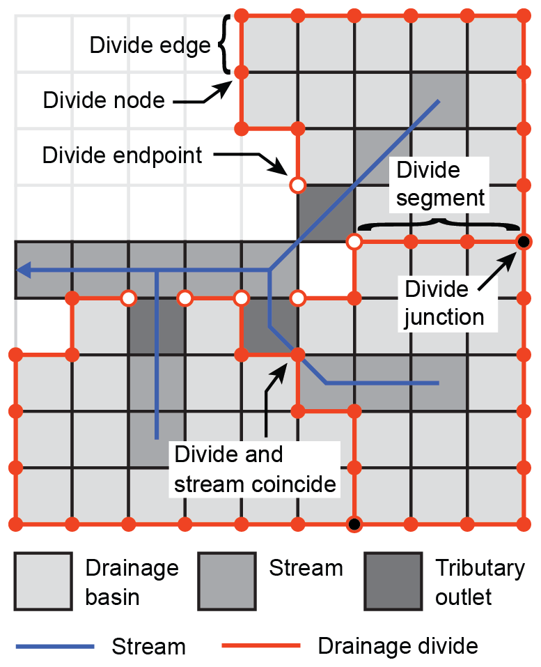
Figure 2Definition of drainage divides in a digital elevation model. Note the point where a drainage divide (red) coincides with a river channel (blue). See text for details.
2.2 Drainage divide networks
Analogous to streams, drainage divides are typically organized into tree-like networks (Fig. 1), although cycles that correspond to internally drained basins may exist. Because of the directed flow of water, stream networks can be regarded as directed graphs that start at channel heads (the leaves of the tree) and end at an outlet or a river mouth (the root of the tree). Flow directions in stream networks can be easily derived from node elevations (e.g., O'Callaghan and Mark, 1984), and the hierarchy of streams can be related to their upstream area, for example. In contrast, drainage divides have no inherent direction, and there is no terrain property, like elevation, that could be used to assign a direction to them. A meaningful metric for ordering divides may be the average branch length (Lindsay and Seibert, 2013), i.e., the average distance Λ (m) one would have to travel down on either side of a divide to reach a common stream location (Fig. 3). However, measuring this distance requires that the common stream location and the entire path leading to it be contained in the DEM. Because this may not be true for a significant part of the divide network in a DEM and because measuring this distance is computationally expensive (Lindsay and Seibert, 2013), it is not very practical.

Figure 3Ordering of divides based on the average distance to a common stream location, Λ. Numbered circles are places on drainage divides (black lines), and blue lines indicate the flow path to their common stream location (red circle). The resulting order of the drainage divide places is . The landscape shown is part of the Big Tujunga drainage basin.
Instead, we suggest that directions can be derived from the tree-like structure of drainage divide networks. Analogous to a parcel of water that travels down a river from its source to its mouth, we propose starting at the leaves of the tree, which we call the endpoints of the divide network (Fig. 2), and incrementally move down the branches (Fig. 4). Note that the term “move down” does not refer to elevation but to the hierarchy of the divide network. Where two or more drainage divides meet, they form a junction. We call individual parts of drainage divides that link endpoints and junctions, junctions and junctions, or endpoints and endpoints the drainage divide segments, and we refer to the ends of divide segments as segment termini to avoid confusion with endpoints. At junctions with more than one unsorted divide segment, the sorting process pauses because it is not obvious in which direction the sorting shall continue. However, in the absence of cycles (internally drained basins), each junction will reach a point in the sorting loop when there is only one unsorted divide segment left so that the sorting can continue (Fig. 4). This condition ensures that the divide segments are correctly sorted in a tree-like manner, but it fails when encountering a cycle. As we will show later, the average branch length Λ scales linearly with the maximum distance from an endpoint along the sorted divide network and the maximum number of divide segments (or junctions), both of which are more easily computed. We thus propose ordering the nodes and edges of the divide network by their maximum distance from divide endpoints, measured either in map units or in the number of divide segments. From now on, we call the distance measured in map units along the directed divide network the divide distance (dd).
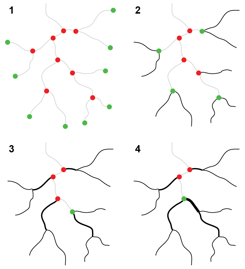
Figure 4Iterative sorting and ordering of the divide network. The divide network is assembled starting with divide segments that contain endpoints (green) and which are then removed from the collection of divide segments. Former junctions (red) that have only one segment remaining become endpoints, and the iteration continues until no more endpoints exist.
3.1 Divide algorithm
We implemented the above-described way of extracting and ordering drainage divides from a DEM in the TopoToolbox v2 (Schwanghart and Scherler, 2014), a MATLAB-based software for topographic analysis. Figure 5 shows the workflow of our approach, which consists of the following steps.
-
For a given DEM, we first define a stream network based on the D8 flow direction algorithm and a threshold drainage area (Fig. 5a, b). The lower the threshold, the more detailed the stream and divide networks will be.
-
We extract drainage divides based on drainage basin boundaries that we obtained for drainage areas at tributary junctions and drainage outlets (Fig. 5c). Initially, each drainage basin boundary is composed of one divide segment that connects two endpoints, and junctions do not yet exist. These divide segments do not cross any rivers but their nodes may coincide with stream edges (Fig. 2). We remove redundant divide segments in the collection of divides, which arise from nested and adjoining drainage basins. As a result, we are left with a set of unique divide segments, which, however, may be continuous across junctions or terminate where they should be continuous (Fig. 6).
-
We next organize the collection of divide segments into a drainage divide network (Fig. 5d). This is the core of the algorithm, in which we identify endpoints and junctions, merge broken divide segments, and split divide segments at junctions (Fig. 6). Our algorithm distinguishes between junctions, endpoints, and broken divide segments by computing for each node of the divide network the number of edges linked to it, the number of segment termini linked to it, and the existence and direction of a diagonal flow direction. For example, most nodes with two edges and two segment termini correspond to a broken segment and need to be merged, unless they coincide with a stream and merging them would make the resulting divide cross that stream (Fig. 6). See the Appendix for more details.
-
Finally, we sort the drainage divide segments within the network (Fig. 5e). The algorithm iteratively identifies segments that are connected to endpoints and removes them from the list of unsorted divide segments until no divide segments are left (Fig. 4). This step assigns a direction to each divide segment and transforms the divide network into a directed acyclic graph. For the sorted divide network, we then compute the divide distance, i.e., the maximum distance from an endpoint along the sorted divide network (Fig. 5f).

Figure 5Workflow of identifying and ordering drainage divides in digital elevation models. (a) Digital elevation model of the Big Tujunga catchment, San Gabriel Mountains, California. (b) Drainage network based on a minimum upstream area of 1000 pixels (0.9 km2). (c) Drainage divides of all drainage basins upstream of confluences in panel (b). (d) Drainage divide network with endpoints (red) and junctions (green). (e) Sorted drainage divide network. Line thickness indicates divide order from low (thin) to high (thick). (f) Drainage divide network color-coded by divide distance (blue: low, yellow: high). Note that only divides at a distance >1 km are shown.
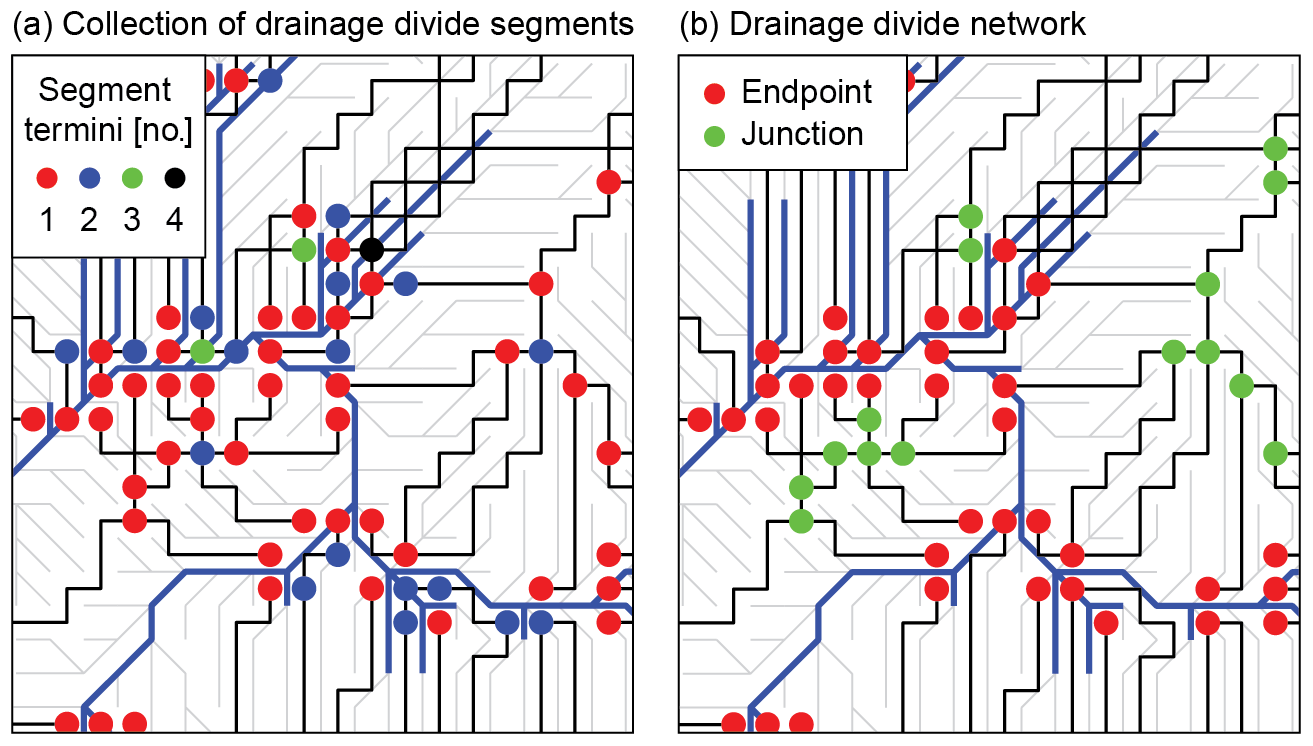
Figure 6Transformation of a collection of drainage divide segments (a) into a drainage divide network with endpoints and junctions (b). Black lines are drainage divides, blue lines are streams, and flow directions are shown as light gray lines. Note that we used a minimum upstream area of only 10 pixels to define the stream network for illustration purposes.
After the sorting, we also assign orders to divide segments based on the ordering of stream networks, first introduced by Horton (1945). We adopted both the Strahler (1954) and Shreve (1966) rules of stream ordering and added a third rule that we call Topo. All ordering schemes start with a value of 1 at endpoints and progressively update divide orders at junctions based on the following rules:
where ωi represents the divide orders of the n joining divide segments, and ωk is the divide order of the following divide segment. In the Strahler ordering scheme, the order increases by 1 if the joining divide segments have the same order; otherwise, it remains at their maximum order. In the Shreve ordering scheme, the resulting divide order is the sum of those of the joining divide segments, and in the Topo ordering scheme, divide orders increase by 1 at each junction. Junctions typically link three different divide segments, but up to four can occur (Fig. 6). Based on the Strahler ordering scheme, the bifurcation ratio Rb can be derived from (Horton, 1945)
where Nω is the number of divide segments of order ω.
As previously mentioned, our divide algorithm currently does not handle internally drained basins. Whereas the divides of internally drained basins are easy to identify, they are not easily sorted in a meaningful manner. In fact, the distance to a common stream location (Λ) is undefined for a divide of an internally drained basin. At the moment, the sorting procedure (Fig. 4) stops at such divides because the divide segments cannot be assigned a direction. In consequence, parts of the divide network that potentially lie beyond an internally drained basin, and for which the distance to a common stream location is defined, can also no longer be reached. While we are working on a solution to this issue, our algorithm is currently best applied to acyclic drainage divide networks.
3.2 Topographic data and analysis
We investigated basic characteristics of drainage divide networks using a 30 m resolution DEM from the 1 arcsec Shuttle Radar Topography Mission data set (Farr et al., 2007). We focused on the catchment of the Big Tujunga River in the San Gabriel Mountains, USA. The catchment is a good example of a transient landscape with active drainage basin reorganization and landscape rejuvenation as the river incises into a relict pre-uplift landscape (DiBiase et al., 2015). We preprocessed the DEM by carving through local sinks (Soille et al., 2003) to avoid artificial internally drained basins, and we obtained a stream network based on a minimum upstream area of 0.1 km2. We note that this threshold is likely well within the zone of debris flow instead of fluvial incision (Stock and Dietrich, 2003), but for the purpose of our analysis, this is irrelevant.
We analyzed the divide network, its planform geometry, and its relation to topography. Planform geometry is studied using statistical analysis of the number and length of divide segments of different orders. Topographic analyses are based on metrics that we determined for the entire DEM and that we subsequently associated, or mapped, to divide edges and entire divide segments. As topographic metrics, we focus on hillslope relief (HR) and horizontal flow distance to the stream network (FD). HR was defined to be the elevation difference between a point on the divide and the point on the river that it flows to. To quantify the morphologic asymmetry of a divide, we propose using the across-divide difference in hillslope relief (ΔHR), normalized by the across-divide sum in hillslope relief (∑HR), and call its absolute value the divide asymmetry index (DAI):
The DAI ranges between 0 for entirely symmetric divides and 1 for the most asymmetric divides. Note that this index is based only on values of hillslope relief (HR). Theoretically, a divide with equal amounts of HR on either side of a divide, but contrasts in flow distance (FD) and thus slope angle, would yield a DAI of zero. However, due to the definition of streams by a minimum drainage area, this hardly ever occurs. In addition, such cases can be identified by cross-divide differences in FD.
4.1 Basic divide statistics
We applied our divide algorithm to the Big Tujunga catchment, and the resulting divide network for different ordering schemes is shown in Fig. 7. Because the Shreve and Topo ordering schemes yield larger ranges in divide orders, their visualization allows for greater differentiation compared to the Strahler ordering scheme. Differences in the visual appearance of the divide network due to the ordering scheme are also apparent at the root node, i.e., the junction that is encountered last in the ordering process (black arrows in Fig. 7). In the Topo ordering scheme, divide orders increase by 1 during each sorting cycle so that the last divide segments will have orders that are different by not more than 1. In contrast, the ordering rules of the Strahler and Shreve schemes (see Eqs. 1 and 2) may yield unequal orders during the sorting so that the divide orders of the last divide segments may be different by more than 1. In the Big Tujunga catchment, the basin area, and thus the number of divide segments, is larger north of the Big Tujunga River compared to south of it. As a consequence, both the Strahler and Shreve divide orders increase more rapidly along the northern perimeter compared to the southern, and the junction encountered last during the sorting process (at the root of the tree) opposes divide segments with orders of 7 and 6 for Strahler and 1463 and 772 for Shreve in the north and south, respectively (Fig. 7). For the Strahler ordering scheme, the frequency distribution of divide segments decreases exponentially with divide order (ω), which is consistent with Horton's law of stream numbers (Horton, 1945), and corresponds to a bifurcation ratio of (standard error). The bifurcation ratio of the associated stream network is 5.39±0.87.
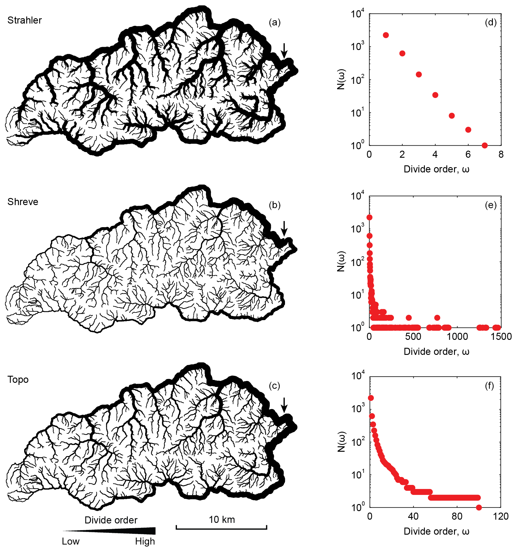
Figure 7Divide network of the Big Tujunga catchment in the western San Gabriel Mountains, California, USA. Panels (a)–(c) show the divide network, with line thickness indicating the divide order. Arrow marks the last divide segment encountered in the sorting process or, equivalently, the root of the tree-like network. Panels (d)–(f) show the number of divide segments as a function of divide order.
We computed divide-segment lengths for different drainage area thresholds (Amin) and show the associated empirical distribution functions in Fig. 8a. Divide-segment lengths are not normally distributed but can be reasonably fitted with a gamma distribution. However, the fitted gamma distributions predict systematically higher probabilities for shorter divide segments and lower probabilities for longer divide segments compared to the actual data. For the different drainage area thresholds that we tested, the shape parameter of the fitted gamma distribution (k) attains values that range between 0.87 and 1.75. In general, the average length of all divide segments increases with the drainage area threshold used for deriving the stream network simply because both the stream and the divide network extend to finer branches. For a drainage area threshold of 0.1 km2, the average length across all divide orders is 442±323 m (±1σ) compared to an expected value (kθ) of ∼442 from the fitted gamma distribution. The average length for different divide orders tends to be slightly lower at (based on the Topo ordering scheme) compared to (Fig. 8b).
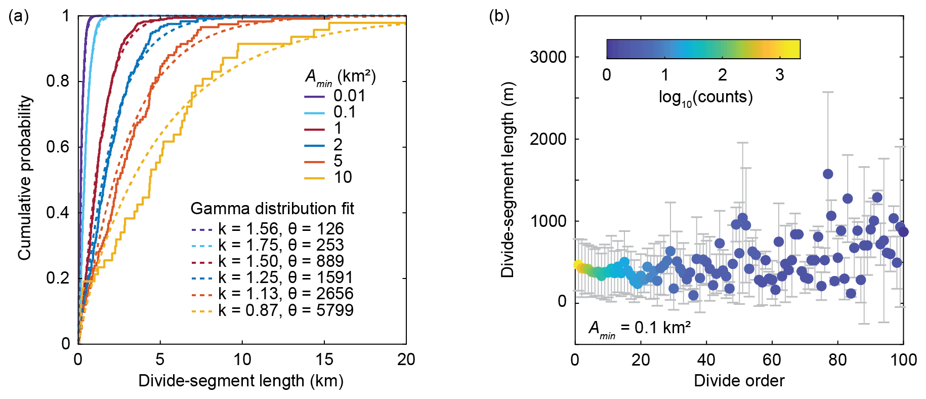
Figure 8Divide-segment statistics. (a) Empirical distribution functions of divide-segment lengths for different drainage area thresholds (Amin) and fitted cumulative gamma distribution functions. (b) Average length (±1σ) of drainage divide segments by order (Topo ordering scheme). The number of observations per divide order drops below 10 at an order of 25.
We quantified the average branch length, i.e., the average distance one would have to travel down on either side of a divide to reach a common stream location (Λ), for 100 randomly chosen divide edges per divide order in the Topo ordering scheme. Although the maximum order for which Λ can be determined (because of the size of our DEM) is limited to ω≤55, results demonstrate that Λ (km) increases linearly as 0.36× divide order (ω) and 1.11× divide distance (dd) (Fig. 9). The linear scaling of these two relationships is a consequence of the similarity of segment lengths for different divide orders (Fig. 8b). Whereas the Topo ordering scheme can be approximated by dividing the divide distance by the expected divide-segment length, this does not hold true for the Strahler and Shreve ordering schemes, which yield relationships between Λ and divide order that are nonlinear (not shown).
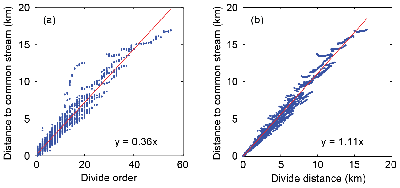
Figure 9Distance to common stream location by (a) divide order and (b) divide distance for 100 randomly chosen divide edges per divide order within the Big Tujunga catchment.
4.2 Drainage divide network morphology of the Big Tujunga catchment
We next studied the morphology of the drainage divide network from the Big Tujunga catchment. Because the divide morphology consists of parts that lie within the catchment and parts that lie outside it, we analyzed the entire drainage divide network from the DEM as shown in Fig. 5. Although the drainage divide network is truncated along the DEM edges, the following analysis is insensitive to this issue. Figure 10 shows the drainage divide morphology of the Big Tujunga catchment based on a stream network that was derived from a drainage area threshold of 1 km2. Topographic metrics are shown for each divide edge (Fig. 10). Whereas across-divide mean flow distance () varies between 0 and ∼3000 m, mean hillslope relief () varies between 0 and ∼800 m. It is notable that the biggest range in values occurs at divide distances <10 km, whereas divides at higher distances appear to hover around characteristic values that are controlled by the drainage area threshold used to derive the stream network (Fig. 10e). It should be noted that divide edges at low divide distances are much more abundant compared to those at higher distances or, equivalently, at higher divide orders (Fig. 7). At increasingly higher drainage area thresholds, however, the frequency of divides at low order and distance decreases more rapidly compared to the frequency of high orders and distances. The average (±1σ) and values for a drainage area threshold of 1 km2 are 1325±350 and 341±129 m, respectively. The empirically determined average values for all tested drainage area thresholds are consistent with Hack's law (Hack, 1957), which relates the length L of the longest stream in a catchment to its drainage area A according to L=kaAh. Values of ka and h are ∼1.6 and ∼0.5, respectively, which are similar to values observed elsewhere (Hack, 1957). Combining and yields average slope values that vary between ∼20 and ∼8∘ for drainage area thresholds between 0.1 and 10 km2. The mean slope value of the entire DEM is ∼21.5∘, which suggests that the lower drainage area threshold better confines the divides to hillslopes compared to lower-sloping channels.
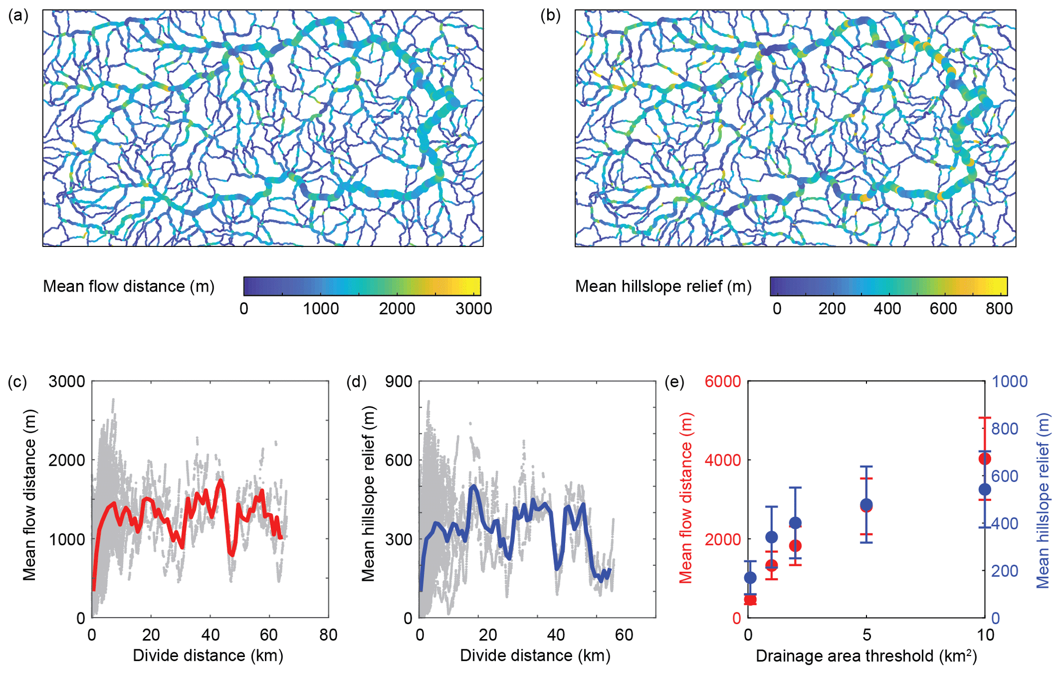
Figure 10Drainage divide morphology of the Big Tujunga catchment based on a stream network that was derived from a drainage area threshold of 1 km2. (a) Drainage divide network (DDN) colored by mean flow distance. Line thickness scales with divide distance. (b) DDN colored by mean hillslope relief. (c) Relationship between mean flow distance and divide distance of all divide edges in panel (a). The red line shows a 1000 m moving average. (d) Relationship between mean hillslope relief and divide distance of all divide edges in panel (b). The blue line shows a 1000 m moving average. (e) Average (±1σ) values of mean flow distance (red) and mean hillslope relief (blue) for different drainage area thresholds. Average values were determined from all divide edges at a divide distance >5 km to minimize the influence of divides that are close to streams simply due to their proximity to confluences.
Based on the observation of characteristic values of and , we sought to identify parts of the divide network that have anomalously low relief or are anomalously close to a stream. Instead of mean values, we turned towards across-divide minimum values of flow distance (FDmin) and hillslope relief (HRmin), as these would be more sensitive to deviations on either side of a divide. In addition, we compared these values with the divide asymmetry index (DAI), as we expected that anomalous divides may also be topographically asymmetric (e.g., Whipple et al., 2017). Figure 11 shows how HRmin, FDmin, and DAI vary with distance along the divide network of the Big Tujunga catchment. Notable deviations from average values (Fig. 10) occur at ∼22–25, ∼41–45, and >54 km divide distance and are typically associated with asymmetric divides (Fig. 11). Highly asymmetric divides are furthermore found at low divide distances (<5 km) and typically coincide with low values of HR, whereas FD could be high or low. The systematic decrease in FD and HR, concurrent with an increase in the DAI at higher divide distances, prompted us to query the geographic position of these divides and how they compare to the surrounding landscape. We thus imposed thresholds to identify anomalously low ( m) and asymmetric divides (DAI >0.5), which are less than 1000 m from a stream ( m) (Fig. 12). Beheaded streams as well as sharp-crested and shortened hillslopes identified in high-resolution satellite imagery (Fig. 12b–e) support the impression that these divides are mobile and migrating in the direction of lower HR and sometimes shorter FD. Most of these divides can be seen to border regions of contrasting local relief (Fig. 12a), and many cluster along the eastern edge of the catchment. The predicted migration direction indicated in Fig. 12a is derived from the orientation of the divide segments and their mean DAI magnitude. If correct, most of the divide migration along the southern and eastern edge of the catchment, from higher to lower relief, would result in area loss for the Big Tujunga catchment.

Figure 11Minimum hillslope relief (a) and minimum flow distance (b) along the divide network of the Big Tujunga catchment. Colors denote the divide asymmetry index (DAI). Black stippled lines indicate the thresholds used to identify anomalous divides in Fig. 12. Gray-shaded areas highlight regions with anomalously low hillslope relief and flow distance.
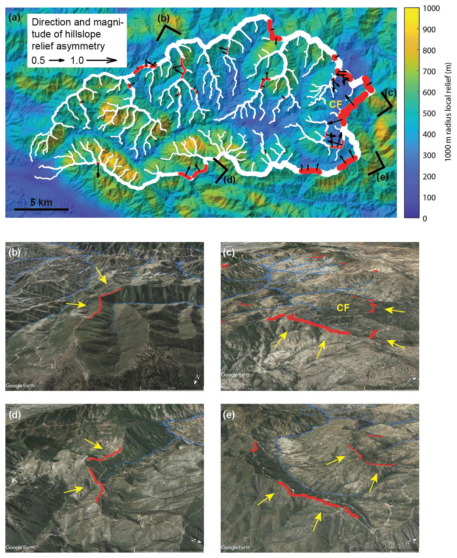
Figure 12Anomalous divides in the Big Tujunga catchment. (a) A 1000 m radius local relief map draped over the hillshade image. White lines show the divide network, and red lines depict asymmetric (DAI >0.4) divide edges with minimum hillslope relief <200 m and minimum flow distance <1000 m. Black arrows indicate the direction and magnitude of the DAI, with the arrow pointing in the direction of lower relief, i.e., the inferred direction of divide migration. (b–e) Oblique Google Earth© views of asymmetric divides shown in panel (a). CF: Chilao Flats.
5.1 Extraction and ordering of drainage divide networks
Our new approach allows for routinely extracting drainage divides from any DEM without internally drained basins. We have shown that the maximum divide distance dd, calculated as the maximum distance along the (directed) divide network from an endpoint, is a meaningful metric for ordering drainage divide networks, as it scales linearly with the average branch length Λ, i.e., the average distance one would have to travel down on either side of a divide to reach a common stream location (Fig. 9). In contrast to the average branch length, however, the divide distance is more easily and rapidly calculated and is less prone to edge effects that inhibit the ordering of divides (Lindsay and Seibert, 2013). However, whenever a drainage basin intersects the edge of a DEM, its truncation will likely produce a spurious drainage divide. Furthermore, calculated divide distances are most likely lower than they would be for a larger DEM, similar to the reduction of upstream area along a stream network. Truncated drainage basin boundaries should therefore be avoided or discarded from analyses that rely on correct divide distances.
The proposed sorting procedure (Fig. 4) recovers the tree-like structure of the divide network and allows for the derivation of divide orders, analogous to the well-known stream orders. Because divide segments have similar mean lengths across all divide orders (Fig. 8), divide orders derived with the Topo ordering scheme can serve a similar purpose as divide distance. Shreve (1969) studied link lengths in stream networks and concluded that their distribution is better described with a gamma distribution compared to an exponential or lognormal distribution. Results from the Big Tujunga catchment support this conclusion with respect to divide-segment lengths, although systematic deviations can be observed (Fig. 8a). It needs to be tested with more observations whether these deviations are inherent to drainage divide networks in general and whether they could hold clues about the dynamic state of a landscape.
An advantage of characterizing the divide network by distance instead of orders is that the divide distance is invariant with respect to the chosen drainage area threshold, whereas divide orders are not because they depend on the total number of divide segments and junctions. Further differences are apparent at the root node, which may oppose divide segments with orders that differ by more than 1 (Fig. 7). In the case of the Big Tujunga catchment, Strahler orders are not that different across the root node, but in a different landscape that could well be the case. This issue is more prevalent in the case of Shreve ordering, but it is avoided with the Topo ordering scheme. Furthermore, the nonuniform distribution of divide-segment lengths (Fig. 8) influences how similar or dissimilar the divide distances of the meeting divide segments are at the root node. If the average divide-segment length of trees that meet at the root node are different, divide distances will make a jump, even if divide orders are similar. In the Big Tujunga catchment, the divide distance jump at the root node is 5400 m.
Divide orders derived with the Strahler ordering scheme can be used to investigate how the divide network conforms to the Horton (1945) laws of network composition. In the Big Tujunga catchment, for example, the bifurcation ratio of the divide network (Rb∼3.9) is lower than that of the stream network (Rb∼5.4). This may in part be due to the fact that we analyzed only a part of the divide network; divide segments that originate from the main catchment boundary and extend outwards are not included in the statistics. Including those in the calculation yields Rb∼4.6 for the divide network, which is still lower than the bifurcation ratio of the stream network. Nevertheless, these bifurcation ratios are similar to published bifurcation ratios of different natural stream networks (e.g., Tarboton et al., 1988), supporting the expected similarity of the stream and divide network topology. However, more observations from different landscapes are needed to assess systematic differences and commonalities between divide and stream networks.
5.2 Drainage divide mobility in the Big Tujunga catchment
Based on the observation of characteristic values of minimum hillslope relief (300–500 m) and minimum flow distance (1000–1800 m), we identified drainage divides in the Big Tujunga catchment that are anomalously low, close to a stream, and asymmetric (Figs. 11, 12). These geometric properties suggest the existence of wind gaps, hillslope undercutting by rivers, and spatial anomalies in erosion rates, which are diagnostic for past or ongoing mobility of drainage divides. Anomalous drainage divides are particularly frequent along the eastern edge of the catchment, where an area of low hillslope angles and local relief (Fig. 12), the so-called Chilao Flats, is bordering a steep catchment to the south and east of it. This high-elevation low-relief area is thought to represent a relict peneplain surface that was uplifted during the growth of the San Gabriel Mountains and is currently being destroyed by the headward incision of rivers (Spotila et al., 2002; DiBiase et al., 2015). Cosmogenic 10Be-derived erosion rates confirm lower erosion rates in the Chilao Flats area compared to the surrounding steeper catchments (DiBiase et al., 2010), which ought to drive divide migration and drainage area loss in the headwaters of the Big Tujunga catchment, consistent with our results.
We identified another stretch of anomalous divides along the southern margin of the Big Tujunga catchment (Fig. 12a, d), part of which is coincident with the trace of the San Gabriel Fault, which follows the orientation of the valley (Morton and Miller, 2006). Reduced relief in a ∼1 km wide zone around this fault is also observed farther to the east along the West Fork of the San Gabriel River (Scherler et al., 2016), suggesting weaker rocks closer to the fault (e.g., Roy et al., 2015). Other anomalous divides in this area, as well as along the northern margin of the Big Tujunga catchment, show signs of mobility by one-side-shortened hillslopes and beheaded valleys (Fig. 12b, d). We thus suggest that most, if not all, of the anomalous divides we identified based on hillslope relief, flow distance, and divide asymmetry are in fact unstable and migrating with time. Because most of the peripheral divides indicate drainage area loss of the Big Tujunga catchment, these area changes ought to result in changes in stream power (Willett et al., 2014), which complicate the interpretation of stream profile knickpoints in a tectonic framework (DiBiase et al., 2015).
In this study, we presented an approach to objectively extract and analyze drainage divides from DEMs. We argued that divides can be ordered in a meaningful way based on the average distance one would have to travel down on either side of a divide to reach a common stream location, and we have shown that this distance can be well approximated by the maximum along-divide distance from endpoints of the divide network, which we termed the divide distance. We have also shown that the tree-like structure of divide networks lends itself to topological analysis similar to stream networks, and we introduced an ordering scheme (Topo), in which divide orders increase by 1 at divide junctions. Because divide segments tend to have characteristic lengths, the Topo ordering scheme mimics the divide distance. Topographic analysis of the drainage divide network of the Big Tujunga catchment yielded characteristic values of flow distance and hillslope relief that can be shown to depend on the drainage area threshold, with which the stream network was derived. Based on these characteristic values and a minimum divide distance of ∼5 km, below which we observed large scatter, we identified divides that have anomalously low hillslope relief, are close to rivers, and are asymmetric in shape. We interpret these divides to be mobile and indicating beheaded valleys or future capture events.
Once the drainage divides are defined based on the outline of drainage basins and redundant divide segments are removed, they compose a network , which is defined by a set of vertices V (or nodes) and a set of edges E, each of which is associated with two distinct vertices. However, D may contain some divide segments that do not end at junctions or that terminate at nodes that are neither junctions nor endpoints. To create the divide network, we have to identify divide endpoints and junctions, as well as divide segments that need to be merged or parted. We achieve this by computing for each node xi the number of edges (1 to 4) and divide-segment termini (0 to 4) that exist in D and identifying whether the node coincides with a stream edge (0∕1) (Table A1). Based on these criteria, we classify nodes to be an endpoint (EP), junction (J), or broken segment (BS). In the case of nodes with three edges, three segment termini, and the presence of a stream edge, we also check which of these edges, if connected, would cross a stream to distinguish the EP from the BS. After this classification, we are able to merge broken segments, split segments at junctions, and thus update D, which now contains all the divide segments that compose the drainage divide network.
Table A1Divide node classification matrix.
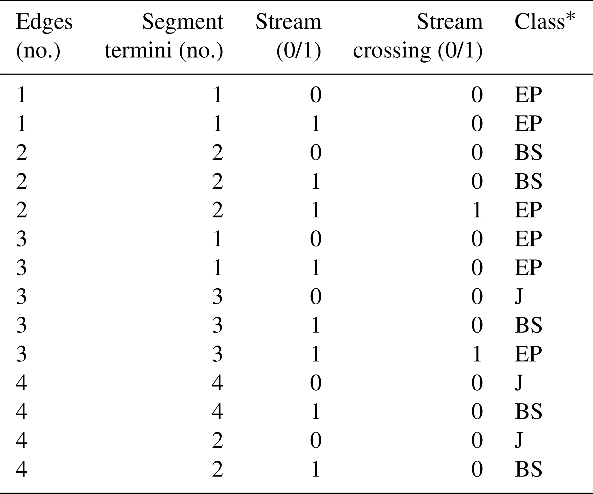
∗ EP: endpoint, BS: broken segment, J: junction.
The divide algorithm developed in this study has been implemented in the TopoToolbox v2 (Schwanghart and Scherler, 2014). The codes will be made available with the next TopoToolbox release and shall be accessible at https://github.com/wschwanghart/topotoolbox (last access: 17 April 2020).
DS developed the algorithm and led the writing of the paper. Both authors contributed to discussions, editing, and revising the paper.
The authors declare that they have no conflict of interest.
We thank two anonymous reviewers for constructive comments that helped improve the paper.
This research has been supported by the Deutsche Forschungsgemeinschaft (DFG; grant no. SCHE 1676/4-1).
The article processing charges for this open-access
publication were covered by a Research
Centre of the Helmholtz Association.
This paper was edited by Sebastien Castelltort and reviewed by two anonymous referees.
Armitage, J. J.: Short communication: flow as distributed lines within the landscape, Earth Surf. Dynam., 7, 67–75, https://doi.org/10.5194/esurf-7-67-2019, 2019.
Beeson, H. W., McCoy, S. W., and Keen-Zebert, A.: Geometric disequilibrium of river basins produces long-lived transient landscapes, Earth Planet. Sc. Lett., 475, 34–43, https://doi.org/10.1016/j.epsl.2017.07.010, 2017.
Bonnet, S.: Shrinking and splitting of drainage basins in orogenic landscapes from the migration of the main drainage divide, Nature Geosci., 2, 766–771, https://doi.org/10.1038/NGEO666, 2009.
Buscher, J. T., Ascione, A., and Valente, E.: Decoding the role of tectonics, incision and lithology on drainage divide migration in the Mt. Alpi region, southern Apennines, Italy, Geomorphology, 276, 37–50, https://doi.org/10.1016/j.geomorph.2016.10.003, 2017.
Castelltort, S., Goren, L., Willett, S. D., Champagnac, J. D., Herman, F., and Braun, J.: River drainage patterns in the New Zealand Alps primarily controlled by plate tectonic strain, Nat. Geosci., 5, 744–748, https://doi.org/10.1038/ngeo1582, 2012.
Clark, M. K., Schoenbohm, L., Royden, L. H., Whipple, K. X., Burchfiel, B. C., Zhang, X., Tang, W., Wang, E., and Chen, L.: Surface uplift, tectonics, and erosion of eastern Tibet as inferred from large-scale drainage patterns, Tectonics, 23, TC1006, https://doi.org/10.1029/2002TC001402, 2004.
Clift, P. D., Blusztajn, J., and Duc, N. A.: Large-scale drainage capture and surface uplift in eastern Tibet–SW China before 24 Ma inferred from sediments of the Hanoi Basin, Vietnam, Geophys. Res. Lett., 33, L19403, https://doi.org/10.1029/2006GL027772, 2006.
DiBiase, R. A., Whipple, K. X., Heimsath, A. M., and Ouimet, W. B.: Landscape form and millennial erosion rates in the San Gabriel Mountains, CA, Earth Planet. Sc. Lett., 289, 134–144, https://doi.org/10.1016/j.epsl.2009.10.036, 2010.
DiBiase, R. A., Whipple, K. X., Lamb, M. P., and Heimsath, A. M.: The role of waterfalls and knickzones in controlling the style and pace of landscape adjustment in the western San Gabriel Mountains, California, Geol. Soc. Am. Bull., 127, 539–559, https://doi.org/10.1130/B31113.1, 2015.
Farr, T. G., Rosen, P. A., Caro, E., Crippen, R., Duren., R., Hensley, S., Kobrick, M., Paller, M., Rodriguez, E., Roth, L., Seal, D., Shaffer, S., Shimada, J., Umland, J., Werner, M., Oskin, M., Burbank, D., and Alsdorf, D.: The Shuttle Radar Topography Mission, Rev. Geophys., 45, RG2004, https://doi.org/10.1029/2005RG000183, 2007.
Fehr, E., Andrade Jr., J. S., da Cunha, S. D., da Silva, L. R., Herrmann, H. J., Kadau, D., Moukarzel, C. F., and Oliveira, E. A.: New efficient methods for calculating watersheds, J. Stat. Mech., 2009, P09007, https://doi.org/10.1088/1742-5468/2009/09/P09007, 2009.
Fehr, E., Kadau, D., Andrade Jr., J. S., and Herrmann, H. J.: Impact of perturbations on watersheds, Phys. Rev. Lett., 106, 048501, https://doi.org/10.1103/PhysRevLett.106.048501, 2011.
Forte, A. M. and Whipple, K. X.: Criteria and tools for determining drainage divide stability, Earth Planet. Sc. Lett., 493, 102–117, https://doi.org/10.1016/j.epsl.2018.04.026, 2018.
Forte, A. M., Whipple, K. X., and Cowgill, E.: Drainage network reveals patterns and history of active deformation in the eastern Greater Caucasus, Geosphere, 11, 1343–1364, https://doi.org/10.1130/GES01121.1, 2015.
Gallen, S. F.: Lithologic controls on landscape dynamics and aquatic species evolution in post-orogenic mountains, Earth Planet. Sc. Lett., 493, 150–160, https://doi.org/10.1016/j.epsl.2018.04.029, 2018.
Gilbert, G. K.: Geology of the Henry Mountains. USGS Report, Government Printing Office, Washington, D.C., USA, 1877.
Goren, L., Castelltort, S., and Klinger, Y.: Modes and rates of horizontal deformation from rotated river basins: Application to the Dead Sea fault system in Lebanon, Geology, 43, 843–846, https://doi.org/10.1130/G36841.1, 2015.
Guerit, L., Goren, L. Dominguez, S., Malavieille, J., and Castelltort, S.: Landscape `stress' and reorganization from χ-maps: Insights from experimental drainage networks in oblique collision setting, Earth Surf. Proc. Land., 43, 3152–3163, https://doi.org/10.1002/esp.4477, 2018.
Hack, J. T.: Studies of longitudinal profiles in Virginia and Maryland, U.S. Geol. Surv. Prof. Pap., 294-B, 1, United States Government Printing Office, Washington, USA, 1957.
Haralick, R. M.: Ridges and Valleys on Digital Images, Comput. Vision Graph., 22, 28–38, 1983.
Horton, R. E.: Erosional development of streams and their drainage basins; hydrophysical approach to quantitative morphology, Geol. Soc. Am. Bull., 56, 275–370, 1945.
Koka, S., Anada, K., Nomaki, K., Sugita, K., Tsuchida, K., and Yaku, T.: Ridge detection with the steepest ascent method, Procedia Comput. Sci., 4, 216–221, https://doi.org/10.1016/j.procs.2011.04.023, 2011.
Lindsay, J. B. and Seibert, J.: Measuring the significance of a divide to local drainage patterns, Int. J. Geogr. Inf. Sci., 27, 1453–1468, https://doi.org/10.1080/13658816.2012.705289, 2013.
Little, J. J. and Shi, P.: Structural lines, TINs, and DEMs, Algorithmica, 30, 243–263, https://doi.org/10.1007/s00453-001-0015-9, 2001.
Morton, D. M. and Miller, F. K.: Geologic Map of the San Bernardino and Santa Ana Quadrangles, California: U.S. Geological Survey Open-File Report 2006–1217, Version 1.0, scale 1 : 100 000, available at: http://pubs.usgs.gov/of/2006/1217 (last access: 5 May 2016), 2006.
O'Callaghan, J. F. and Mark, D. M.: The extraction of drainage networks from digital elevation data, Comput. Vision Graph., 28, 323–344, https://doi.org/10.1016/S0734-189X(84)80011-0, 1984.
O'Hara, D., Karlstrom, L., and Roering, J.J.: Distributed landscape response to localized uplift and the fragility of steady state, Earth Planet. Sc. Lett., 506, 243–254, https://doi.org/10.1016/j.epsl.2018.11.006, 2019.
Ranwez, V. and Soille, P.: Order independent homotopic thinning for binary and grey tone anchored skeletons, Pattern Recogn. Lett., 23, 687–702, https://doi.org/10.1016/S0167-8655(01)00146-5, 2002.
Roy, S. G., Koons, P. O., Upton, P., and Tucker, G. E.: The influence of crustal strength fields on the patterns and rates of fluvial incision, J. Geophys. Res.-Earth, 120, 275–299, https://doi.org/10.1002/2014JF003281, 2015.
Scherler, D. and Schwanghart, W.: Drainage divide networks – Part 2: Response to perturbations, Earth Surf. Dynam., 8, 261–274, https://doi.org/10.5194/esurf-8-261-2020, 2020.
Scherler, D., Lamb, M. P., Rhodes, E. J., and Avouac, J.-P.: Climate-change versus landslide origin of fill terraces in a rapidly eroding bedrock landscape: San Gabriel River, California, Geol. Soc. Am. Bull., 128, 1228–1248, https://doi.org/10.1130/B31356.1, 2016.
Schwanghart, W. and Heckmann, T.: Fuzzy delineation of drainage basins through probabilistic interpretation of diverging flow algorithms, Environ. Modell. Softw., 33, 106–113, https://doi.org/10.1016/j.envsoft.2012.01.016, 2012.
Schwanghart, W. and Scherler, D.: Short Communication: TopoToolbox 2 – MATLAB-based software for topographic analysis and modeling in Earth surface sciences, Earth Surf. Dynam., 2, 1–7, https://doi.org/10.5194/esurf-2-1-2014, 2014.
Shreve, R.: Statistical law of stream numbers, J. Geol., 74, 17–37, 1966.
Shreve, R.: Stream Lengths and Basin Areas in Topologically Random Channel Networks, J. Geol., 77, 397–414, https://doi.org/10.1086/628366, 1969.
Soille, P., Vogt, J., and Colombo, R.: Carving and adaptive drainage enforcement of grid digital elevation models, Water Resour. Res., 39, SWC-10.1-13, https://doi.org/10.1029/2002WR001879, 2003.
Spotila, J. A., House, M. A., Blythe, A. E., Niemi, N. A., and Bank, G. C.: Controls on the erosion and geomorphic evolution of the San Bernadino and San Gabriel Mountains, southern California, in: Contributions to Crustal Evolution of the Southwestern United States: Boulder, Colorado, eidted by: Barth, A., Geological Society of America Special Paper, 365, 205–230, 2002.
Stock, J. and Dietrich, W. E.: Valley incision by debris flows: Evidence of a topographic signature, Water Resour. Res., 39, 1089, https://doi.org/10.1029/2001WR001057, 2003.
Strahler, A. N.: Statistical analysis in geomorphic research, J. Geol., 62, 1–25, 1954.
Tarboton, D. G.: A new method for the determination of flow directions and upslope areas in grid digital elevation models, Water Resour. Res., 33, 309–319, https://doi.org/10.1029/96WR03137, 1997.
Tarboton, D. G., Bras, R. L., and Rodriguez-Iturbe, I.: The fractal nature of river networks, Water Resources Res., 24, 1317–1322, 1988.
Whipple, K. X., Forte, A. M., DiBiase, R. A., Gasparini, N. M., and Ouimet, W. B.: Timescales of landscape response to divide migration and drainage capture: implications for the role of divide mobility in landscape evolution, J. Geophys. Res.-Earth, 122, 248–273, https://doi.org/10.1002/2016JF003973, 2017.
Willett, S. D., McCoy, S. W., Perron, J. T., Goren, L., and Chen, C. Y.: Dynamic reorganization of river basins, Science, 343, 1248765, https://doi.org/10.1126/science.1248765, 2014.
Yang, R., Willett, S. D., and Goren, L.: In situ low-relief landscape formation as a result of river network disruption, Nature, 520, 526–529, https://doi.org/10.1038/nature14354, 2015.