Ice-Hot News : The “Oldest Ice” quest has begun

There is million-year old ice somewhere deep under the surface of the Antarctic ice sheet! [Credit: Brice Van Liefferinge]

This is it! The new European horizon 2020 project on Oldest Ice has been launched and the teams are already heading out to the field, but what does “Old Ice” really mean? Where can we find it and why should we even care? This is what we (Marie, Olivier and Brice) will try to explain somewhat.

Why do we care about old ice, ice cores and past climate?

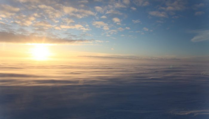
Figure 1: Drilling an ice core [Credit: Brice Van Liefferinge]

Unravelling past climate and how it responded to changes in environmental conditions (e.g. radiative forcing) is crucial for our understanding of the current climate and for predicting how climate will likely change in the future.

Ice cores contain unique and quantitative information on the past climate (e.g. atmospheric gas concentration). The caveat is that at the moment, we can “only” go back up to 800,000 years at EPICA Dome C ice core (Parrenin et al, 2007).

Nonetheless, marine records tell us that during the Mid-Pleistocene there was a major climate transition (0.8-1.2 million years ago): a change in the frequency of glacial-interglacial cycles in the Northern Hemisphere. Instead of an ice age every 40,000 year, the climate changed to what is termed a “100,000 year world”. Unfortunately, the time resolution of marine records are too coarse to provide details on the mechanisms behind such climate changes. We must therefore rely on ice cores to obtain a high enough temporal resolution. Furthermore, the ice traps air bubbles and can therefore provide a record of the atmospheric composition that can be used to directly measure the paleo atmosphere through the transition.

The new European project ‘Oldest ice’ was set up for this very objective: crack the Mid-Pleistocene Transition climate. It brings together engineers, experimentalists and modellers from 14 Universities around the world.

In this post, we will focus on the first mission of the project: locating areas with million year old ice in Antarctica. The next steps will be to:

• develop the drilling technology,

• improve our geophysical knowledge of the identified site,

• and finally, reach the “holy grail”: recover ice from the very base of the ice sheet with a target age of 1.5 Million years.

The whole project is anticipated to last 10 years!

The new European project ‘Oldest ice’ was set up for this very objective: crack the Mid-Pleistocene Transition climate

The first mission: “Where to find million year old ice?”

Oldest Ice (ice more than 1 mio. years old) can only be recovered in Antarctica, but where exactly? This question has to be answered in a two-step approach:

1. On a large scale, we must first narrow down places in Antarctica where Oldest Ice might be found. To do that, we rely on models.

2. Then, we can focus our analysis on those regions by gathering field data in the form of airborne radar surveys. Further ground-based work is currently taking place.

On a larger scale, Oldest Ice in Antarctica requires:

1. Thick ice and cold bed. We need thick ice to reconstruct past climate variations with sufficient temporal resolution (e.g. is there enough ice to measure air bubbles or other climate markers). However, the thicker the ice, the higher the basal temperature. If the bottom of the ice is too warm, the ice at the base will start to melt, potentially destroying the Oldest Ice of the ice sheet.
   Finding a suitable drill site hence requires a good trade-off between thickness and cold-bed conditions.

2. Slow-moving ice. This is found mainly at the centre of the ice sheet. Imagine this: if ice were to flow at as little as 1 m per year over a period of 1.5 Million years, it would have travelled 1,500 km over that time interval! However, there is a catch: slow-moving areas are also low-accumulation areas, and low accumulation means warmer ice. This is because the ice is cooled by the addition of cold snow at the surface that then gets transformed to ice and then travels downwards. Indeed, the greater the accumulation, the deeper the “cold snow” can penetrate into the ice sheet!

3. Undisturbed ice. In order to obtain an interpretable climate record, the ice recovered from the drill needs to be stratigraphically ordered, i.e. no mixing of the ice can have occurred so that we can assume that time increases with depth when we measure ice composition down the core. Variations in the height of the bedrock can induce such ice mixing.

(more information can be found in Van Liefferinge and Pattyn (2013))

Figure 2. Potential locations of cold bed (basal temperatures 2000 m), slow motion (horizontal flow speeds <2m/yr) The colour bar represents the basal temperature. The two insets focus on Dome C and Dome F, two areas highly likely to store million year old ice. [Credit: Brice Van Lieffering, updated from Van Liefferinge, B. and Pattyn, 2013]

While boundary conditions such as ice thickness and accumulation rates are relatively well constrained, the major uncertainty remains in determining thermal conditions at the ice base. The thermal conditions depend on the geothermal heat flow (the flux of “energy” provided by the Earth which conducts heat into the crust) underneath the ice sheet. But to measure the geothermal heat flow, you need to reach the bed.

We need to find the ideal drilling location which would satisfy all these conditions – a bit of a “Goldilocks’ choice”: thick ice but not too much, low accumulation but not too low, low geothermal heat flow but high enough to not get folded basal ice. To do this we use several models: a simple one which calculates the minimum geothermal heat flow needed to reach the pressure melting point that we can then compare to data sets, and a more complex one resolving in three dimensions the temperature field with thermomechanical coupling (i.e. linking the ice-flow component to the heat-flow component). The combination of modelling approaches shows that the most likely oldest ice sites are situated near the ice divide areas (close to existing deep drilling sites, but in areas of smaller ice thickness) (see Figure 2).

Give it a go: Try to find million year old ice yourself using this Matlab© tool: http://homepages.ulb.ac.be/~bvlieffe/old-ice.html

The combination of modelling approaches shows that the most likely oldest ice sites are situated near the ice divide areas

On finer scales: we need deep radiostratigraphy and age modelling

Radar profiles

Figure 3. Radargram from the new Oldest Ice A radar survey (Young et al., in review) with isochrones interpreted in red [Credit: Marie Cavitte]

Radargrams (see figure 3) are powerful tools to observe the internal structure of the ice: variations in density, acidity and ice fabric all can create conductivity contrasts, which result in radar visual stratigraphy. Below the firn column (the compacting snow, up to 100 m thick), most returns are related to acidity variations, corresponding to successive depositional events (i.e. snowfall). Radar stratigraphy in this case can be considered isochronal, i.e. every visible line (see figure 3) were formed at the same moment, (Siegert et al., 1999). Such radar isochrones can then be traced for kilometres throughout the ice sheet where radar data has been acquired. When radar lines intersect an ice core site, the radar stratigraphy can then be dated by matching the isochrone-depths to the ice core depths at the site and then transferring the age-depth timescale.

This allows to date entire sub-regions. However, the very bottom of the ice column is often difficult to interpret: radar isochrones cannot always be continuously followed from the ice core.

Radargrams are powerful tools to observe the internal structure of the ice

The newly acquired Oldest Ice A radar survey (Young et al., in review) over the Dome C region (see figure 2 for location) gives very rich stratigraphic information and the proximity of the EPICA Dome C ice core has allowed the dating of the isochrones. The ice sheet in this area could only be dated to ~360,000 years (Cavitte et al., 2016) and not further back in time because deeper isochrones are tricky to tie to the ice core, and other times, there is no clear signal (deep scattering ice, visible near the bedrock, at the bottom of Figure 3). As such, we need an age model to try to describe the age-depth relation below the deepest dated isochrones.

Modelling the ice

Figure 4. More precise analysis of the Dome C Oldest Ice target, with the lines representing the Oldest Ice A airborne survey collected in winter 2015/16 (Young et al., in review). The colours represent the modelled age of the ice 60 meters above the bedrock, in thousands of years. We can see that this whole region has a lot of potential for recovering million year old ice. [Credit: Olivier Passalacqua]

The age of the ice primarily depends on its vertical velocity, so we can use a simple 1D model to describe the motion of the ice in the vertical direction. We run the model for an ensemble of vertical velocity profiles and basal melt rates, and consider the distribution of the basal ages (i.e. model ages) given by the profiles that reproduce the observations the best (i.e. isochrones ages).

We need an age model to try to describe the age-depth relation below the deepest dated isochrones

After running the model, it appears that many areas of the Oldest Ice A survey region host very old ice (see red and yellow dots on figure 4 which represent ages > 1 million years). A high enough bottom age gradient, provided by the dated isochrones, is required to ensure sufficiently old ice as a drilling target. Following initial calculations, it will probably be a better choice to drill on the flank of the bedrock relief than on its top.

So in the end, where do we find the oldest ice?

We have to find areas which provide a good compromise between thick ice (for the a good temporal resolution in the ice core) but not too thick (to avoid basal melting). The best sites will be the ones close to the surface ridge (to ensure limited displacement of the ice), standing above the surrounding subglacial lakes, and for which a lot of undated isochrones below the last dated isochrone are visible.

To find out more about Beyond EPICA and keep track of progress visit the project  website and follow @OldestIce on twitter!

Edited by Sophie Berger

Brice Van Liefferinge is a PhD student and a teaching assistant at the Laboratoire de Glaciology, Université libre de Bruxelles, Belgium. His research focuses on the basal conditions of the Antarctic ice sheet. He tweets as @bvlieffe.

Marie Cavitte is a PhD student at the Institute for Geophysics at the University of Texas at Austin, Texas. Her research focuses on understanding radar internal stratigraphy and using it as a means to constrain the temporal stability of the East Antarctic Ice Sheet interior.

Olivier Passalacqua is a PhD student at the Laboratoire de Glaciologie et Géophysique de l’Environnement, Grenoble, France.

Members of the consortium

• Alfred Wegener Institute, Helmholtz Centre for Polar and Marine Research (AWI, Germany), Coordination
• Institut Polaire Français Paul Émile Victor (IPEV, France)
• Agenzia nazionale per le nuove tecnologie, l’energia e lo sviluppo economico sostenibile (ENEA, Italy
• Centre National de la Recherche Scientifique (CNRS, France)
• Natural Environment Research Council – British Antarctic Survey (NERC-BAS, Great Britain)
• Universiteit Utrecht – Institute for Marine and Atmospheric Research (UU-IMAU, Netherlands)
• Norwegian Polar Institute (NPI, Norway)
• Stockholms Universitet (SU, Sweden)
• Universität Bern (UBERN, Switzerland)
• Università di Bologna (UNIBO, Italy)
• University of Cambridge (UCAM, Great Britain)
• Kobenhavns Universitet (UCPH, Denmark)
• Université Libre de Bruxelles (ULB, Belgium)
• Lunds Universitet (ULUND, Sweden)

Non-Europan partners

• Institute for Geophysics, University of Texas at Austin (UTIG, US)
• Australian Antarctic Division (AAD, Australia)