We have waited eight years for it, and it is finally out: the 6th Assessment Report of the Intergovernmental Panel on Climate Change (a.k.a. « IPCC AR6 »)! And it is more than 10,000 pages long across Working Groups! Fortunately, a synthesis report integrating the findings of all three working groups should be released in Autumn 2022. However, we, at the EGU Cryosphere Blog, thought it might be useful to highlight the main cryo-findings!
A brief history of the IPCC
Before diving into the science, let’s start with a brief reminder of the context. “What is the IPCC?”, “What exactly can we find in an assessment report?”, “How many scientists are involved in writing an assessment report?”, “Are the authors paid to write it?”, you know, the casual questions that usually come up in conversations…
The Intergovernmental Panel on Climate Change (in short: IPCC) was established in 1988 by the United Nations (UN) to inform UN members on the origin and consequences of climate change. The IPCC mission is to “prepare a comprehensive review and recommendations with respect to the state of knowledge of the science of climate change; the social and economic impact of climate change, and potential response strategies and elements for inclusion in a possible future”. Since then, six so-called “assessment reports” (in 1990, 1995, 2001, 2007, 2013/14 and 2021/22) have been published (see Figure 2).
To address its diverse missions, the IPCC produces three assessment reports in one cycle, each prepared by a different “Working Group”, and one synthesis report. Working Group 1 (WG1) reviews “The Physical Science Basis”, Working Group 2 (WG2) reviews “Impacts, Adaptation, and Vulnerability” and Working Group 3 (WG3) reviews “Mitigation of Climate Change”. Additionally, governments can ask for more focused reports in terms of topic, such as for example the “Special Report on Global Warming of 1.5°C” and the “Special Report on the Ocean and Cryosphere in a Changing Climate”. In these special reports, elements touching the competencies of all three Working Groups are included.
In an IPCC assessment report (in short: AR), you will not find any original research. As mentioned before, the role of the IPCC is to summarize and assess the current state of knowledge around climate change. In a world with increasing interest in climate change and high publication output, this means reading and summarizing more than 66,000 scientific publications! For this huge effort, close to 1,000 scientists from all over the world work together for several years. And… they do it “for free”, which means that they are not working full-time for the IPCC and are not paid by it. Instead, they conduct this huge effort in addition to their usual academic life. So, thank you to all the authors and contributors for the time you put into it!
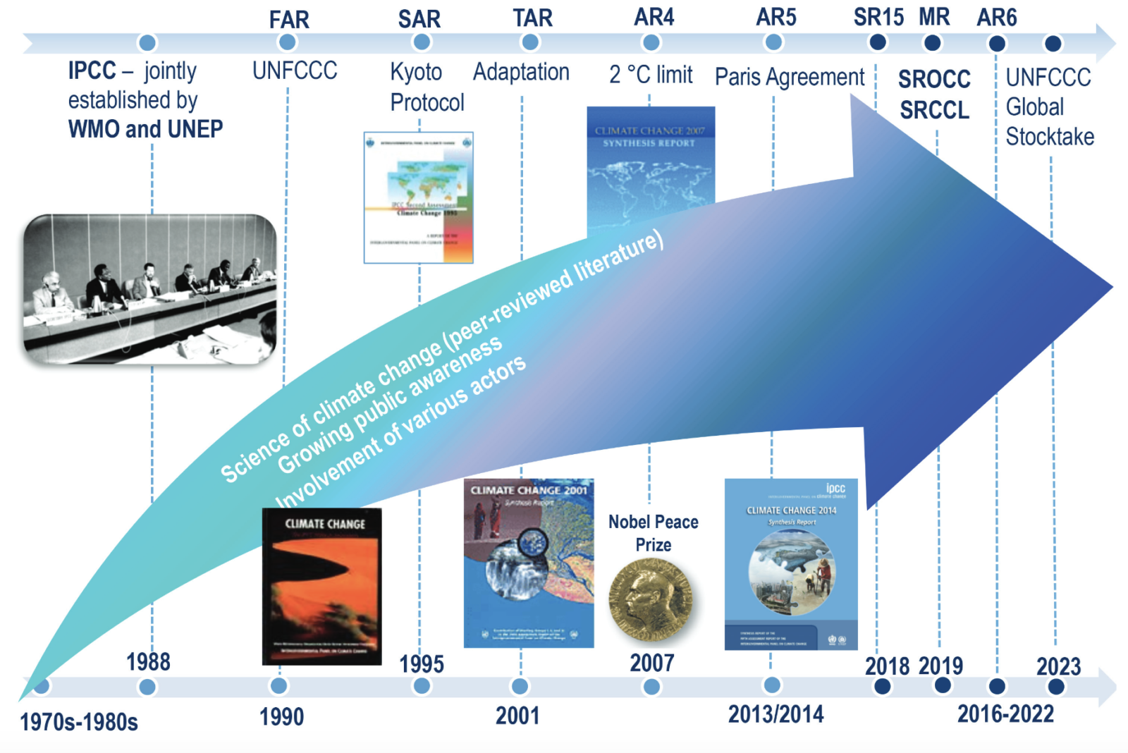
Figure 2: Schematic of the evolution of the IPCC and IPCC assessment reports. Figure credit: IPCC brochure, 2017
The IPCC AR6 – Working Group 1
We, at the EGU Cryoblog, are rather physical science nerds. This is why we mainly focus here on the findings from Working Group 1, in particular the findings related to the cryosphere. If you are interested in an overview over the whole WG1 report, we recommend these two excellent overview articles prepared by Carbon Brief, one in the form of a Questions & Answers, and one presenting the key new insights as seen from scientists.
Basically, the main conclusion of this report is that there is no doubt possible that human activities are driving climate change and that every ton of CO2 that is (and will be) emitted adds to climate change. Also, there were new insights into the attribution of given aspects of climate change to human activities and into more regional aspects of climate change.
Next to the core report, written in complex IPCC “language”, we recommend that you check out the great features that make the conclusions more accessible: the Interactive Atlas, the Frequently Asked Questions (FAQs) or the Regional Fact Sheets! Finally, if you are interested in what happens “behind the curtains” of the IPCC process and are joining the EGU General Assembly, do not hesitate to check out this short course!
Concerning the cryosphere, the IPCC authors and contributors have already worked intensely on it in recent years, as the special report focused on the ocean and cryosphere came out in 2019. Still, science has advanced rapidly, even more greenhouse gasses have been emitted to the atmosphere and the climate has continued to warm. In the following, we summarize the most up-to-date knowledge for the different elements of the cryosphere, as assessed in the IPCC AR6 WG1 report.
Snow
The seasonal snow cover can mainly be found in mountainous regions and at mid to high latitudes. Due to its high albedo, a measure related to its “whiteness”, snow reflects much more sunlight than the surface it covers, which can be ice, grass or bare ground for example. Its presence therefore influences the energy available locally. It is also a good insulator, working like a blanket, so that less heat escapes from the warm ground to the cold air above. Mainly in mountainous regions, snowmelt in spring represents a source of freshwater but also modulates the timing and volume of possible flooding.
The main results from the IPCC report concern the Northern Hemisphere as snow covers nearly 50% of its land surface at its maximum, while it covers less than 5% in the Southern Hemisphere (Antarctica excluded). The terrestrial snow cover is described by three variables: (1) the snow cover extent, (2) the snow cover duration and (3) the accumulation of snow (expressed either through snow depth or snow water equivalent).
New observational products show that the snow cover extent decreased in all months between 1981 and 2018. In some months, this decrease exceeded 50 thousand km² (the size of Slovakia or nearly twice the size of Belgium) per year (see Figure 3) and was tightly linked to global warming. The snow line (the limit at which precipitation falls as snow) migrates upwards in mountains and northward more generally as the climate warms. Also, the snow cover remains for a shorter period, as the snowmelt starts earlier in spring. It is also possible that snow has started to fall later in the year than previously, but it is challenging to robustly observe this period (many clouds and less sun) so no clear conclusion can be drawn about this aspect. And, finally, less and less snow accumulates. The spring snow water equivalent has been decreasing since 1981. For example, for March, it has decreased by 4.6 Gigatons/year (short: Gt/yr), the equivalent of nearly 2 million olympic swimming pools, on average, every year between 1980 and 2018.
Note that these conclusions are drawn at the level of the Northern Hemisphere. The amplitude and sign of the trends can vary widely at the local scale. Additionally, in mountainous terrain, it is more difficult to quantify the changes as variations are very local and high-resolution observations are lacking.
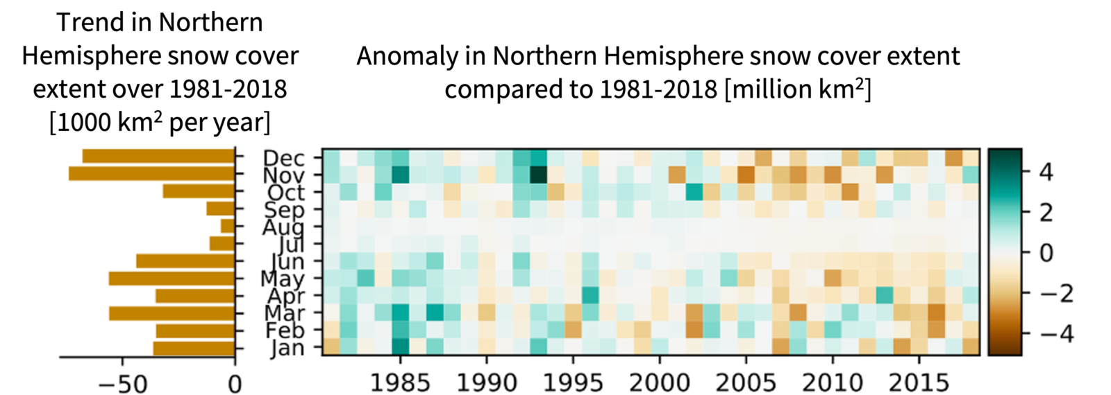
Figure 3: Observed monthly trends (left) and anomalies (right) of snow cover extent in the Northern Hemisphere. Trends and anomalies are calculated over the 1981-2018 period. Figure adapted from IPCC AR6, WGI, Fig. 9.23a) and b).
Snow models have greatly improved since the previous IPCC report (taking into account several snow layers and more physical processes). As a result, snow evolution is better represented in model simulations. These models project that the snow cover will shrink further in the future and that snow will be present for shorter and shorter periods as the global climate continues to warm due to the strong link with temperature changes. Process understanding suggests that this also applies to the Southern Hemisphere.
This is a very short summary of Section 9.5.3. (Seasonal snow cover), with some information from Chapter 8 (Water cycle changes – 8.2.3.1, 8.3.1.3, 8.4.1.3, 8.5.3.2). Check them out for more details!
Glaciers
Apart from the Greenland and Antarctic ice sheets, the world’s land ice is stored in the form of glaciers. Glaciers are large bodies of ice that form from snowfall over many years, often centuries. They move under their own weight due to gravity. There are over 200,000 glaciers in the world, with information about them stored in the Randolph Glacier Inventory. Compared to the ice sheets, glaciers make up a relatively small part of global ice volume (less than 1%), and thus potential global sea level rise (only 0.32 m in case all the ice stored in glaciers melted), but they still heavily influence sea-level rise. Also, they are important freshwater storage vessels and indicators of climate change.
Glaciers are distributed in many places around the world and therefore are subject to different climatic conditions in time and space. Still, on a global scale, glaciers are declining. From 1901 to 1990, glaciers have lost 7 to 28% of their 1901 mass. From 1901 to 2018, the meltwater from glaciers was the dominant contributor to global sea level rise, accounting for 41% of it. In more recent years, the melting of the ice sheets has accelerated and glacier melt accounted for “only” 15.4% of sea-level rise between 2006 and 2018. This doesn’t mean that less meltwater reaches the ocean, just that glacier melt only represents a smaller percentage of the total meltwater now reaching the ocean. Overall, the decade 2010-2019 was the decade of the highest recorded glacier mass loss since the beginning of observations!
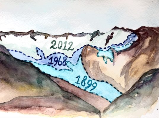
Changes in glacier properties, such as glacier growth and melt or changes in their geometry, are driven primarily by changes in temperature and snowfall. Glaciers shrink when they are in imbalance: they gain less mass, mainly through snowfall, than they lose, mainly through melt. The AR6 report states that humans drive this imbalance, causing the retreat of nearly all glaciers worldwide since the 1990s.
Glacier processes are being observed and simulated more and more accurately, through advances in e.g. satellite images and glacier models. One of the major recent achievements is that we can now estimate glacier retreat for almost all (94%!) glaciers in the world. This dataset, by Hugonnet et al. (2021), shows that over the past 20 years, most glacier retreat was observed in the regions of the Southern Andes, New Zealand, Alaska, Central Europe, and Iceland. Meanwhile, glaciers melt at lower speed in High Mountain Asia, the Russian Arctic, and the periphery of Antarctica.
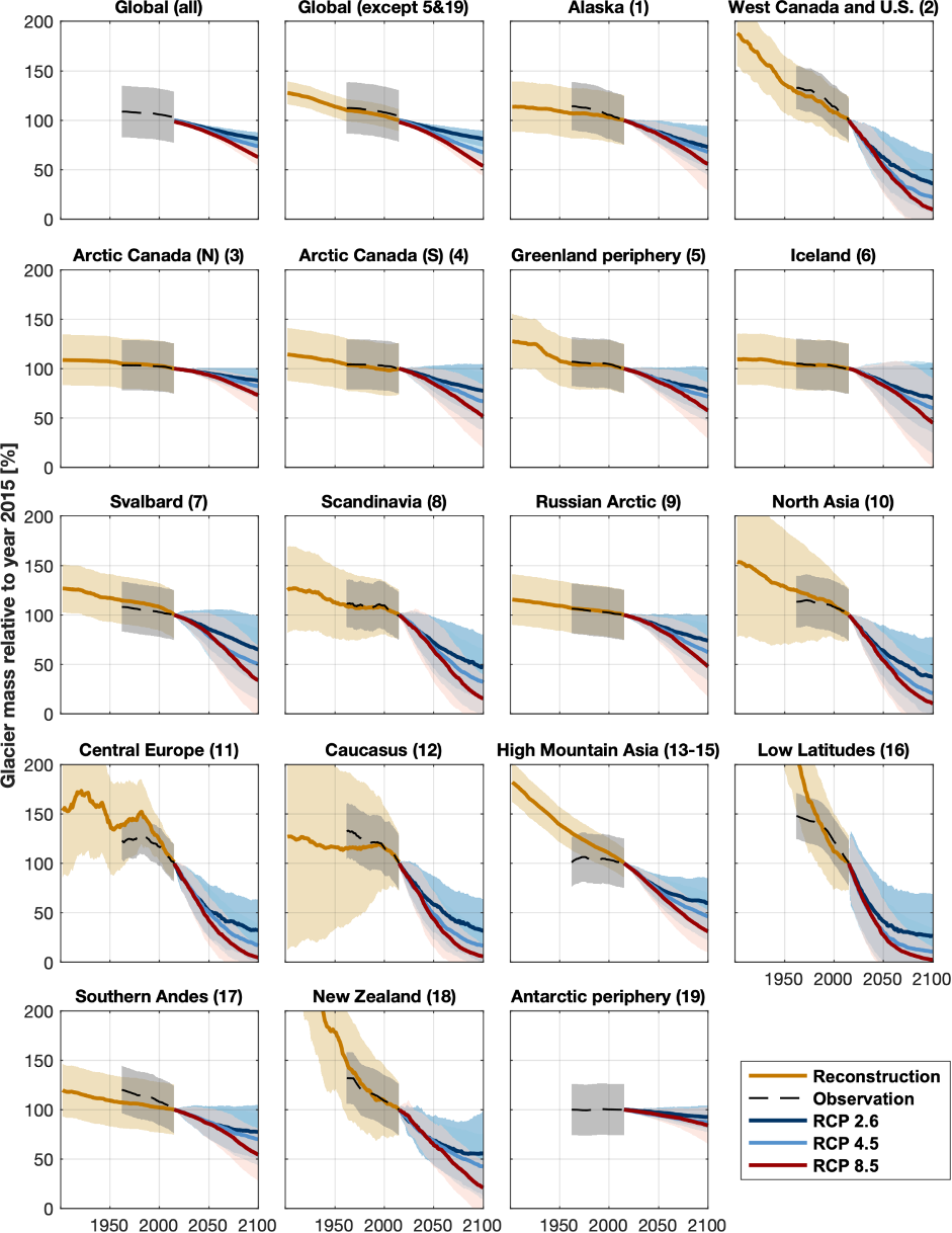
Figure 4: Glacier mass balance over the different regions, from reconstructions, observations and future simulations. As evident from the numbers in the text as well: a clear loss of ice from glaciers. Figure adapted from IPCC, AR6, WG1, figure 9.21.
In the future, glaciers will continue to melt, even if we manage to stabilize global temperatures at some point. Because glaciers respond to changes in climate with a time lag, they will therefore continue to shrink for several decades. Models project that as much as 36% of the glaciers’ ice mass will disappear in any case, just because of the warming that has already happened until now. The full extent of future glacier melt depends on the region, model and climate scenario, but overall, studies agree that we can expect it to continue (Figure 4).
This is a very short summary of Section 9.5.1. (Glaciers). Check it out for more details!
Ice sheets
The large ice sheets that cover Greenland and Antarctica might be far from us but their melting affects us all. If the ice covering Greenland melted away completely, it could lead to a sea-level rise of 7 m in total. If the ice covering Antarctica melted away, we would be talking about almost 60 m as Antarctica is much larger than Greenland!
Currently, there is still a lot of ice left and we are still far from this catastrophic scenario, so don’t panic (yet)! However, even if we stopped emitting greenhouse gasses today, the melting of the ice sheets would not stop right away. This means that sea level will continue to rise in any case in the future (projections until 2100 shown in Figure 5). For example, if we do not exceed 1.5°C of warming (compared to pre-industrial levels), this so-called “committed” rise in sea level ranges from 2 to 3 m in 2000 years to 6 to 7 m in 10,000 years.
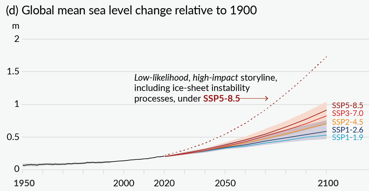
Figure 5: Observed (black) and model projections (colors) of global mean sea level changes (induced by glacier and ice-sheet melt as well as ocean warming) for different so-called SSP scenarios compared to 1900. The higher the number at the end of the SSP-name, the more greenhouse gasses are emitted until 2100. Shades represent uncertainty ranges. Figure credit: IPCC AR6, WGI, Fig. SPM 8d.
Greenland ice sheet
Observations clearly show that the Greenland ice sheet is shrinking faster and faster. It lost on average 39 Gt/yr from 1992 to 1999, which is the equivalent of a cube of ice with 3.5 km-long edges dumped into the ocean every year! From 2000 to 2009, it lost 175 Gt/yr (cube edge of 5.8 km) and, from 2010 to 2019, it lost 243 Gt/yr (cube edge of 6.5 km). The shrinking of the ice sheet can be seen both in the lowering of the surface, through surface melting, and in the retreating ice sheet margins, where the ice sheet meets the ocean. The increase in surface melting is mainly due to the warmer air near the surface. Additionally, it is amplified by the so-called “ice-albedo feedback”, a vicious circle: less and less of the ice sheet is covered by snow, and bare ice is darker than snow. As a consequence, the surface reflects less sunlight, which leads to more ice melt (see this post explaining the sea-ice-albedo feedback). The retreat of the ice sheet margins is mainly driven by submarine melt of marine-terminating glaciers due to warmer ocean temperatures and to surface meltwater that has reached the bottom of the ice sheet and then flowed towards the ocean. Note that, while overall the ice sheet is shrinking, there is a large variability between years in the pace of this retreat.
According to model projections, the Greenland Ice Sheet will continue to lose ice under all emission scenarios in the coming century, contributing 1 to 18 cm to sea-level rise until 2100 compared to 1995-2014. On longer timescales (e.g. until 2300), large uncertainties remain.
Antarctic ice sheet
The Antarctic ice sheet has been losing ice as well over the past decades. From 1992 to 1999, it lost on average 49 Gt/yr (cube of ice with 3.8 km-long edges). From 2000 to 2009, it lost 70 Gt/yr (cube edge of 4.3 km) and, from 2010 to 2016, 148 Gt/yr (cube edge of 5.5 km). Most of this ice loss is a consequence of warmer ocean water getting in contact with the bottom of the ice shelves, principally in West Antarctica. Ice shelves are the huge ice tongues reaching out onto the ocean at the outskirts of the ice sheet and they usually “buttress” the ice flowing towards the ocean, which means that they act like a brake on the ice flow from the ice sheet into the ocean. Due to the warmer ocean, these ice shelves are melting from below, and thinning as well as retreating. Their “braking” effect does not work as well anymore and more ice from inland reaches the ocean, leading to sea-level rise. In East Antarctica, the ice mass has increased in some regions and decreased in others, compensating each other, so that no clear change has been detected overall.
Model simulations of the future evolution of Antarctica are very uncertain, especially because potential instabilities can follow the thinning and retreat of the ice shelves (such as for example the Marine Ice Sheet Instability or the Marine Ice Cliff Instability, see also this IPCC figure). As a consequence, the model projections for 2100 are difficult to quantify. In IPCC language, it is likely that the ice will continue melting throughout the century, with projections ranging from 0 to 63 cm in terms of sea-level rise depending on the scenario and model assumptions. The deep uncertainty around changes in the Antarctic ice sheet makes projections beyond 2100 even less quantifiable.
This is a very short summary of Sections 9.4.1. (Greenland) and 9.4.2. (Antarctica). Check them out for more details!
Sea ice
Sea ice is frozen ocean water, which forms and grows in polar oceans every winter and melts every summer. It is present in both the Arctic and Antarctic, with a reversed timing for maximum and minimum sea-ice coverage due to their opposite locations.
Arctic sea ice
The IPCC AR6 report confirms the large decline in Arctic sea-ice area since the beginning of satellite observations in 1979, with a drop of about 40% in September (when Arctic sea-ice area reaches its minimum) and a decrease of about 10% in March (when Arctic sea-ice area reaches its maximum), when comparing today to 1979. The report also confirms that human influence is the main driver of this decline (see this post for an explanation of the different causes of Arctic sea-ice loss). More than half of the summer sea-ice loss is driven by human-induced global warming, which results from higher greenhouse gas concentrations (see this post for the link between CO2 and Arctic sea ice).
Based on the most recent model projections, the Arctic Ocean could become almost free of sea ice in the summer at least once before 2050 in all emission scenarios. However, if greenhouse gas emissions are drastically reduced, the mean Arctic sea-ice area will stabilize at around 2 million km² in 2050, while it will continue its strong drop until the end of the century if large quantities of greenhouse gasses continue to be emitted (Figure 6). The Arctic Ocean will remain ice-covered in winter in all scenarios during this century, although sea-ice area will decrease over time.
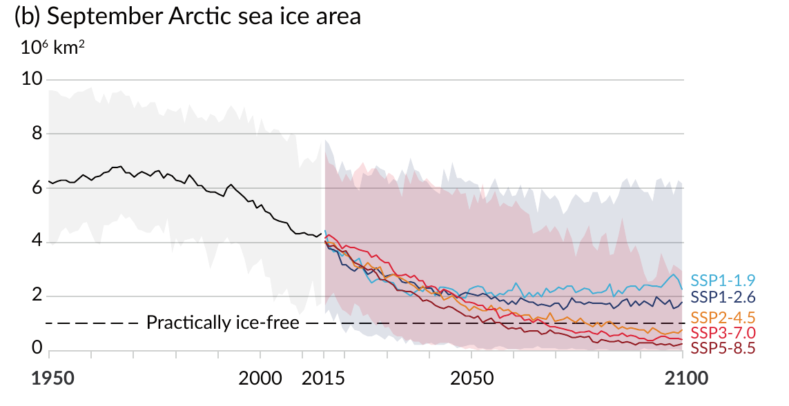
Figure 6: Time evolution of September Arctic sea-ice area from 1950 to 2100 from CMIP6 models; the black curve shows the historical simulation (1950-2014) and the colored curves show 5 different future emission scenarios (2015-2100) Figure credit: Fig. SPM8(b) from the IPCC AR6, WG1 report.
Antarctic sea ice
On the other side of the planet, in Antarctica, there has been no clear change in the sea-ice area from 1979 to now. This absence of change hides in fact a relatively large year-to-year variability, but also regional differences. Some years, like 2022, have exhibited a very strong sea-ice melting, and other years, like 2015, have been marked by below-normal melting. Also, some regions have experienced a small sea-ice gain (e.g. Weddell and Ross Seas) and other regions a small sea-ice loss (e.g. Amundsen Sea).
The IPCC report also claims that there is ‘low confidence in existing future projections of Antarctic sea-ice evolution’ and thus does not provide numbers. This is due to large model uncertainties, limited observations and a lack of process understanding. Let us hope some improvements in these three areas can be done in the near future in order to get a better idea about how Antarctic sea ice will behave.
This is a very short summary of Section 9.3 (Sea ice). Check it out for more details!
Permafrost
Permafrost soils have been frozen “perennially”, which means for at least two years but often thousands of years. The global permafrost region covers 22 million km2 (a little more than twice the size of Canada!). In regions with annual average temperatures below 0°C, dead plants do not decompose. Instead, they, and the carbon they store, accumulate in the frozen soil. As a consequence, Arctic permafrost soils store a large quantity of carbon, equivalent to half of all global carbon contained in soil.
Since the 1980s, permafrost has warmed to record temperatures. And while the global average warming of around 0.3°C between 2007 to 2016 across polar and alpine regions might not seem like a lot, it causes “thermal erosion”, which can occur gradually or abruptly (read our blog post about it here). Every summer season, the “active layer” at the top of the permafrost soil column thaws. With global warming, the active layer is getting gradually deeper (Figure 7). Improvements have been achieved since the last report by the large monitoring programs “Circumpolar Active Layer Monitoring” and “The Global Terrestrial Network for Permafrost”.
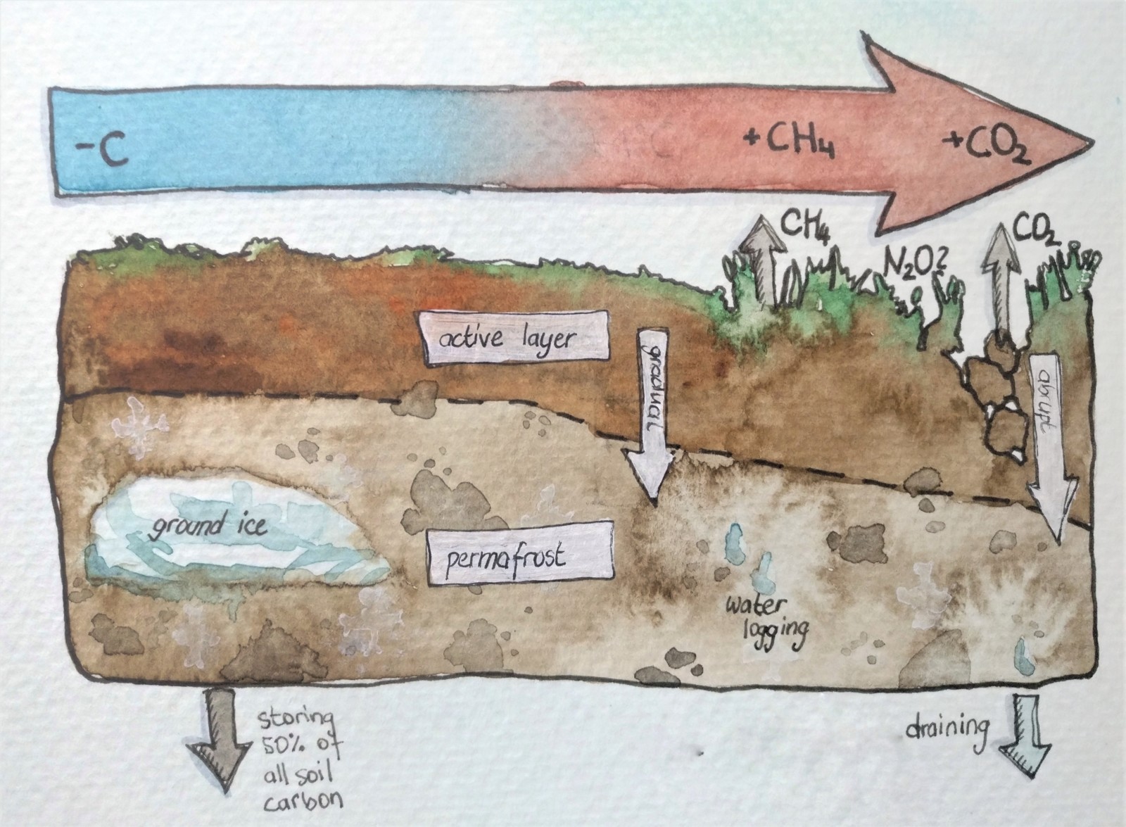
Figure 7: Schematic showing how, with global warming, the active layer deepens or collapses. The thawing releases the stored carbon (C) in the form of the greenhouse gasses CO2, CH4 as well as N2O. Figure credit: Maria Scheel.
On top of these gradual changes, more abrupt changes can take place. The frozen ground can also include huge blocks of ground ice, which can melt in a short time and collapse, creating “thermokarsts” but also unstable ground for houses and streets. Through these deep collapses of the soil surface, formerly protected deep carbon stocks become vulnerable. Now, while it took millennia to form these massive reservoirs, erosion leads to an irreversible release of this ancient carbon to the atmosphere (through biological decomposition and export by freshwater). It is however still uncertain how fast and intense the current permafrost changes are. Also, how much CO2, CH4 and N2O will be emitted cannot be projected confidently yet, as long-term observations are still rare and many factors, such as microbial activity and abrupt permafrost thaw, are just not well studied enough.
This section is based on the Section 9.5.2 (Permafrost) and additional information from Chapter 2 (Changing state of the climate system – 2.3.2.5) and the Technical Summary (TS.3.2.2 and TS.4.3.2.8).
In summary
Most cryosphere components (snow cover, glaciers, ice sheets, sea ice, permafrost) have suffered from the effects of climate change in past decades and will continue to do so in the future. In this post, we did our best to summarize these changes in light of the last IPCC WG1 report. It paints a gloomy picture as global greenhouse gas emissions are not yet decreasing. The next logical question is: what are the future impacts of climate change and what can we do about it, besides continuing to monitor and simulate changes?
Well, part of the answer can be found in the Working Group 2 and 3 reports that came out in February and April 2022, respectively. These are focussed on impacts and adaptation (WG2) and mitigation (WG3) of climate change. Summarizing their main messages in one section would not do them enough honor, especially as their results are a little out of our topic of expertise. Fortunately, other people have taken the time to summarize them, so do not hesitate to check out these great resources:
Working Group 2
- Creative overview in the form of a Twitter thread by @theweirdnwild
- Presentation of the Summary for Policymakers with zero jargon in the form of a Twitter thread by @KANichols
- 16 main messages presented with cats in the form of a Twitter thread by @timparrique
- Questions & Answers put together by Carbon Brief
- Scientist reactions put together by Carbon Brief
Working Group 3
- Some of the most important messages in the form of a Twitter thread by @SarahLynnBurch
- Questions & Answers put together by Carbon Brief
- Scientist reactions put together by Carbon Brief
- EGU Geolog blog – GeoPolicy: Climate solutions at the center of focus this Earth Day
Further reading
- IPCC WG1 website
- Scripts to reproduce the figures from Chapter 9
- How to cite the different parts of the IPCC
- Frequently Asked Questions (FAQs) of WG1 in the form of a Twitter thread by @SoBrgr.
- Short IPCC & cryosphere overview by the International Cryosphere Climate Initiative (ICCI)
- Youtube – IPCC Sixth Assessment Report – The numbers behind the science
We would like to thank Mickaël Lalande for his helpful input for the snow section of this post.
Edited by Sophie Berger and Marie Cavitte

Clara Burgard is a postdoctoral researcher at the Institut des Géosciences et de l’Environnement (IGE) in Grenoble. She currently investigates melt parametrizations at the base of Antarctic ice shelves as part of the H2020 PROTECT project. Before that, she did her PhD on investigating sea ice in climate simulations and comparing it to sea ice observed by satellites. She tweets as @climate_clara.

David Docquier is a post-doctoral researcher at the Royal Meteorological Institute of Belgium. His study focuses on the interactions between the ocean and atmosphere using tools from nonlinear sciences. His work is embedded within the JPI-Oceans/JPI-Climate ROADMAP project.

Maria Scheel is a PhD student at Aarhus University in Denmark. Her current research explores how permafrost microorganisms adapt to the ongoing thaw and erosion in Northeast Greenland. Besides that, she tweets as @Maria_Scheel_ and @mindfulscient.
Larissa van der Laan is a PhD Student at the Leibniz University Hannover, Germany and artist, aiming to communicate climate science (among other things) through art. Her research is within the project GLISSADE, focusing on glacier mass balance modelling on seasonal and decadal scales, using the Open Global Glacier Model (OGGM). Find her artistic and scientific musings on Instagram @anda.designstore and on twitter under @larissavdlaan.