the Creative Commons Attribution 4.0 License.
the Creative Commons Attribution 4.0 License.
 | 13 Mar 2019
Attributing the 2017 Bangladesh floods from meteorological and hydrological perspectives
Sjoukje Philip
Sarah Sparrow
Sarah F. Kew
Karin van der Wiel
Niko Wanders
Roop Singh
Ahmadul Hassan
Khaled Mohammed
Hammad Javid
Karsten Haustein
Friederike E. L. Otto
Feyera Hirpa
Ruksana H. Rimi
A. K. M. Saiful Islam
David C. H. Wallom
Geert Jan van Oldenborgh
In August 2017 Bangladesh faced one of its worst river flooding events in recent history. This paper presents, for the first time, an attribution of this precipitation-induced flooding to anthropogenic climate change from a combined meteorological and hydrological perspective. Experiments were conducted with three observational datasets and two climate models to estimate changes in the extreme 10-day precipitation event frequency over the Brahmaputra basin up to the present and, additionally, an outlook to 2 ∘C warming since pre-industrial times. The precipitation fields were then used as meteorological input for four different hydrological models to estimate the corresponding changes in river discharge, allowing for comparison between approaches and for the robustness of the attribution results to be assessed.
In all three observational precipitation datasets the climate change trends for extreme precipitation similar to that observed in August 2017 are not significant, however in two out of three series, the sign of this insignificant trend is positive. One climate model ensemble shows a significant positive influence of anthropogenic climate change, whereas the other large ensemble model simulates a cancellation between the increase due to greenhouse gases (GHGs) and a decrease due to sulfate aerosols. Considering discharge rather than precipitation, the hydrological models show that attribution of the change in discharge towards higher values is somewhat less uncertain than in precipitation, but the 95 % confidence intervals still encompass no change in risk. Extending the analysis to the future, all models project an increase in probability of extreme events at 2 ∘C global heating since pre-industrial times, becoming more than 1.7 times more likely for high 10-day precipitation and being more likely by a factor of about 1.5 for discharge. Our best estimate on the trend in flooding events similar to the Brahmaputra event of August 2017 is derived by synthesizing the observational and model results: we find the change in risk to be greater than 1 and of a similar order of magnitude (between 1 and 2) for both the meteorological and hydrological approach. This study shows that, for precipitation-induced flooding events, investigating changes in precipitation is useful, either as an alternative when hydrological models are not available or as an additional measure to confirm qualitative conclusions. Besides this, it highlights the importance of using multiple models in attribution studies, particularly where the climate change signal is not strong relative to natural variability or is confounded by other factors such as aerosols.
- Article
(7755 KB) - Full-text XML
-
Supplement
(1289 KB) - BibTeX
- EndNote


In August 2017 Bangladesh faced one of the worst river flooding events in recent history, with record high water levels, and the Ministry of Disaster Management and Relief reported that the floods were the worst in at least 40 years. Due to heavy local rainfall, as well as water flow from the upstream hills in India, the various rivers in northern Bangladesh burst their banks. This led to the inundation of river basin areas in the northern parts of Bangladesh, starting on 12 August and affecting over 30 districts. The National Disaster Response Coordination Centre (NDRCC) reported that around 6.9 million people were affected, with 114 people reported dead and at least 297 250 people displaced. Approximately 593 250 houses were destroyed, leaving families displaced in temporary shelters.
Bangladesh is a highly flood-prone country, with flat topography and many rivers that regularly flood and are used to irrigate crops and for fishing. The August 2017 floods were particularly impactful as they followed two earlier flooding episodes in late March and July that year, increasing the vulnerability of people. Nearly 85 % of the rural population in Bangladesh works directly or indirectly with agriculture, and rice is the main staple food, contributing to 95 % of total food production. As is typical after such flooding, farmers started to plant aman, the monsoon rice that is almost entirely rain dependent. However, the August flood was worse than that of July, and areas such as Dinajpur and Rangpur that normally do not flood were also flooded (see Fig. 1). These are areas that contain significant rice production. As a result, 650 000 ha of croplands were severely damaged during the August monsoon flooding in the year. Aman rice is historically the most variable, and yields tend to drop dramatically during major flood years (Yu et al., 2010). The flood-induced crop losses in 2017 resulted in the record price of rice, negatively affecting livelihood and food security. Beyond impacts to agriculture, the floods destroyed transport infrastructure such as railways lines, bridges and roads, leaving some areas inaccessible to disaster relief efforts. The rise in water and strong current breached roads and embankments and swept away livestock, houses and assets that may have otherwise been protected. At least 2292 schools were damaged, affecting education for weeks, and 13 035 cases of waterborne illnesses were reported in the aftermath of the floods.
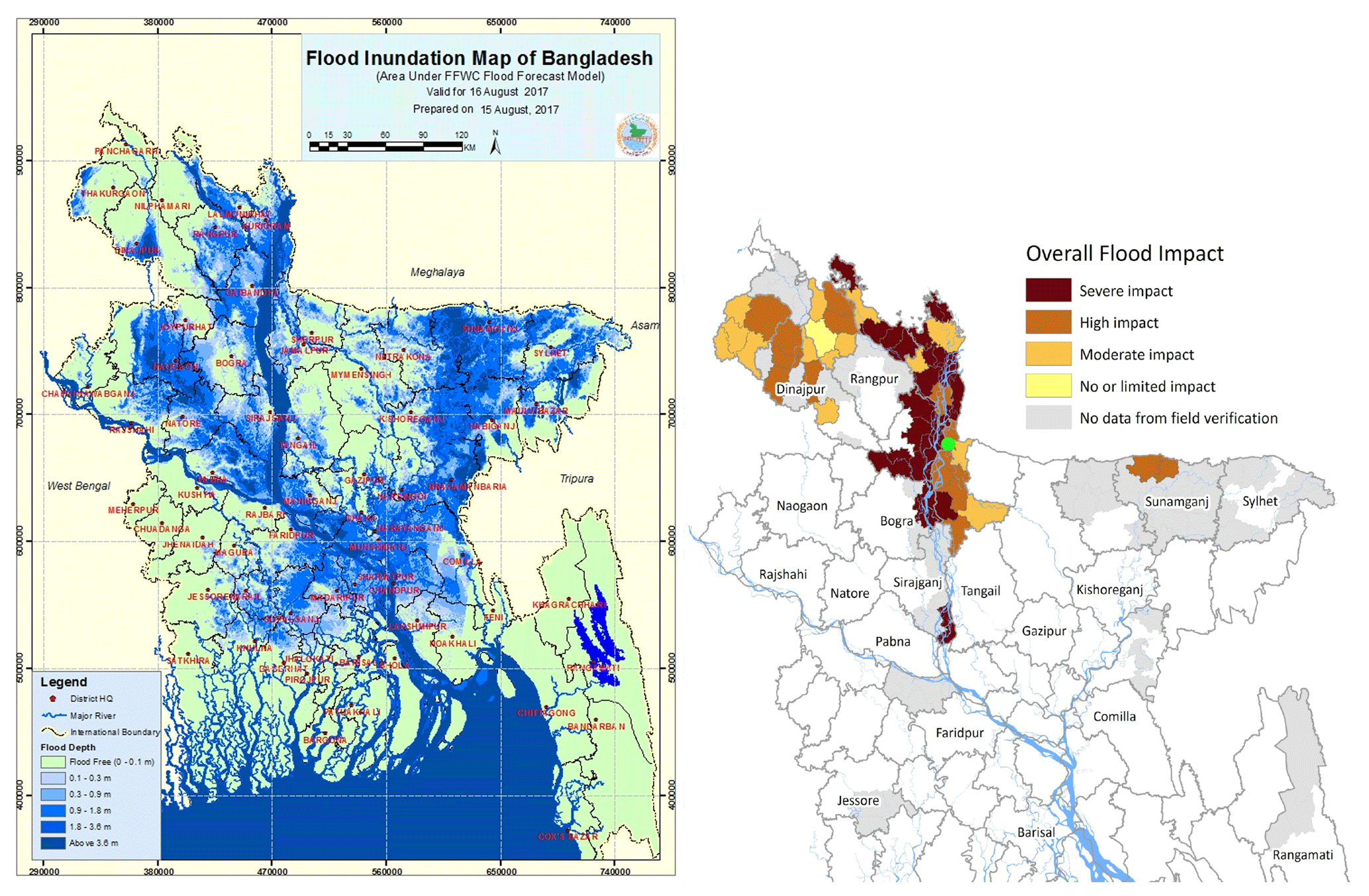
Figure 1Inundation forecast map of Bangladesh for 16 August 2017 (left panel). Overall flood impact of the August 2017 flooding as stated on 21 August (right panel). The green circle in the northwest of the map denotes the location of Bahadurabad. The Brahmaputra basin is outlined in Fig. 3; see the original documents (source: Flood Forecast and Warning Center – FFWC – of BWDB at https://reliefweb.int/sites/reliefweb.int/files/resources/SitRep_2_Bangladesh Flood_16 August 2017.pdf, last access: 8 May 2018 and https://reliefweb.int/sites/reliefweb.int/files/resources/72 hrs-Bangladesh_Flood_Version1_Final 08212017.pdf, last access: 8 May 2018) for more details on the maps and legends.
The 2017 flood was markedly different from previous major flood events in 1988 and 1998, when both the Ganges and Brahmaputra flooded simultaneously (Webster et al., 2010). Based on forecasts it was feared that a similar event would occur in 2017, but in this case, the swelling of the Brahmaputra; its tributary, the Atrai; and the Meghna caused flooding. The worst impacts were along the main reach of the Brahmaputra River (Fig. 1b).
The first estimates of the return period provided by the Bangladesh Water Development Board (BWDB) for the 2017 flood event range from an event occurring once in 30 years to an event occurring once in 100 years, depending on the data source: water level and discharge data at Bahadurabad (the main station for discharge representing the Brahmaputra in Bangladesh) and the flooding forecast system GloFAS. These estimates, however, were implicitly based on the assumption of a stationary climate and did not account for the possibility that the frequency of such flooding events may be changing.
Extreme rainfall events that subsequently lead to widespread flooding, such as the 2017 event in Bangladesh, are one of the main types of extreme weather events that we are expecting to see more of in a warming climate. But with rainfall not only being driven by thermodynamic processes but also being affected by changing atmospheric processes, it is not clear a priori if such events at a particular location will increase in likelihood or if the dynamic changes will mean that the overall chance of extreme rainfall decreases there (Otto et al., 2016). Furthermore, in the current climate, drivers other than greenhouse gases (GHGs) often play a role that is currently difficult to quantify but likely to mask or exacerbate the effect of greenhouse-gas emissions so far on the occurrence likelihood of extreme rainfall events (e.g. aerosols, van Oldenborgh et al., 2016). Hence regional attribution studies are necessary for identifying whether and to what extent extreme rainfall events are changing and for providing insight into which drivers have been contributing to those changes and whether the trend is likely to continue into the future. Attribution studies require both observational data and models to fully estimate the impact of changes in the climate system. The reported advances in model development for the Brahmaputra region and their success in forecasting gives good confidence in the models' ability to accurately represent the region.
Hydrological models are increasingly used for studies on flooding in Bangladesh. As upstream flow data are absent for Bangladesh, a lot of effort has been made to develop flood forecasting systems based on satellite data and weather predictions. Webster et al. (2010), for instance, developed a system that forecasts the Ganges and Brahmaputra discharge into Bangladesh in real time on 1-day to 10-day time horizons. In a recent study Priya et al. (2017) show that, by using a new long lead flood forecasting scheme for the Ganges–Brahmaputra–Meghna basin, skillful forecasts are provided that inherently not only express a prediction of future water levels but also supply information on the levels of confidence with each forecast. Hirpa et al. (2016) used reforecasts to improve the flood detection skill of forecasts.
Previous scientific studies generally show an increasing trend in climate projections of extreme rainfall and high discharge in the region. For example, Gain et al. (2011) use the PCR-GLOBWB model with input from 12 global circulation models (GCMs; 1961–2100) from the CMIP3 ensemble (Meehl et al., 2007) in a weighted ensemble analysis. They show that in this ensemble, there is a positive trend in the peak flow at Bahadurabad; in this model configuration and under the SRES B2 scenario, a peak flow that currently occurs every 10 years will occur at least once every 2 years during the time period 2080–2099. Dastagir (2015) gives an overview of the change in flooding according to the IPCC 5th Assessment Report, using 16 GCMs from the CMIP5 ensemble (Taylor et al., 2012). They state that the warmer and wetter climate predicted for the Ganges–Brahmaputra–Meghna basin by most climate-related research in this region indicates that vulnerability to severe monsoon floods will increase with climate change in the flood-prone areas of Bangladesh. The same conclusion is reached by CEGIS and SEN authors (2013), who use GCM projections and a hydrological model to show that in the wet season, an increase in precipitation and annual flow is projected. In line with this, Mohammed et al. (2017) find that in a 2.0 ∘C warmer world, floods will be both more frequent and of a greater magnitude than in a 1.5 ∘C warmer world in Bangladesh, using the hydrological model the Soil and Water Assessment Tool (SWAT) with input from the CORDEX regional model ensemble. Zaman et al. (2017) use two sets of climate models with climate change runs under the RCP8.5 scenario as input in a basin model that simulates flows in major rivers of Bangladesh, including the Brahmaputra. Using the two climate model runs as input, they find agreement in the basin model runs for Brahmaputra flow in a 2.0 ∘C warmer world; one run shows a slightly higher impact of climate change compared to the other run, with an overall increase in monsoon flow of approximately 15 % and 10 % in the dry season.
Attribution studies on flooding, using both observational data and models, have often been done with precipitation only. In such studies, (e.g. Schaller et al., 2014; van der Wiel et al., 2017; Philip et al., 2018; van Oldenborgh et al., 2017; Risser and Wehner, 2017) it is assumed that precipitation is the main cause of the flooding. For shorter timescales and the relatively small basins involved, this is a reasonable assumption. The major basins in Bangladesh, however, are substantially larger and have longer water travel times than the basins considered in the above studies. Therefore using precipitation alone as a proxy for flooding might not be appropriate. In this paper we explicitly test this assumption by performing an attribution of both precipitation and discharge as a flooding-related measure of climate change. Thus we explore the flood in two different ways – first from a meteorological perspective (using precipitation data) and then from a hydrological perspective (using discharge data). Schaller et al. (2016) already studied a flooding case in an attribution study using one hydrological model. Yuan et al. (2018) use observations, GCMs, and one land surface model with and without land cover change to split the changes in observed streamflow and its extremes into anthropogenic and natural climate change, land cover change and human-water withdrawal components. In this paper we do an attribution study for the first time using observational precipitation and discharge data and a combination of GCMs and several hydrological models. To compare the differences between the attribution results for the two variables we calculate the return periods and risk ratios for the August 2017 flooding event in Bangladesh for both precipitation and discharge in observations and models, for past (pre-industrial), present and future (2∘ warmer than pre-industrial) conditions.
Bangladesh is influenced by three large river basins: the Ganges basin in the northwest, the Brahmaputra basin in the northeast and the Meghna basin in the east. During the monsoon season the rainfall moves northwest across the country, starting in May–June–July in the Meghna basin. Usually 2–3 weeks after peak rainfall in July, the rivers in the Brahmaputra basin reach their peak discharge. Finally, in August and September the Ganges basin river discharge peaks. The largest impact of flooding in August 2017 was felt in the northern parts of Bangladesh (Fig. 1). As this was mainly caused by precipitation in the Brahmaputra basin, the focus in this paper will be on this basin. In the Brahmaputra basin little water originates from precipitation on the northern side of the Himalaya (China–Tibet), with most of the water coming from precipitation in the upstream Assam region in India. Precipitation in Bhutan also contributes to the river water in Bangladesh.
In this paper we use two event definitions: one based on precipitation and one based on discharge. Both observational data and model data can be used for these two event definitions. For precipitation we average over the whole Brahmaputra basin and take a 10-day average, as the largest precipitation volume in the Brahmaputra basin travels to Bangladesh within 10 days; see Fig. 5 in Webster et al. (2010). Only precipitation in July–August–September (JAS) is analysed as it is only in these months that precipitation is considered the major cause of flooding. For discharge we simply use the daily maximum discharge at Bahadurabad, a station situated to the north of the confluence point of the Ganges with the Brahmaputra, in JAS.
The data and methods used are described in Sect. 2. Sections 3 and 4 describe the analysis for observations and models respectively. The results are synthesized in Sect. 5. A discussion follows in Sect. 6, and the paper ends with some conclusions.
Observational data are described in Sect. 2.1, and the models and experiments are described in Sect. 2.2. The explanation of how these data are used in the analysis is detailed in Sect. 2.3.
2.1 Observational data
The first observational dataset we use is the 0.5∘ gauge-based CPC analysis from 1979 to now (https://www.cpc.ncep.noaa.gov/products/Global_Monsoons/gl_obs.shtml, last access: 20 March 2018). This is the longest gauge-based daily gridded dataset available that is still being updated. The seasonal cycle of precipitation in the Brahmaputra basin is shown in Fig. 2a. Monsoon rains start rising slowly, with a maximum in July and August, and become less from September onwards. As precipitation will not, in general, cause flooding before July, we will use the months JAS for the precipitation analysis.
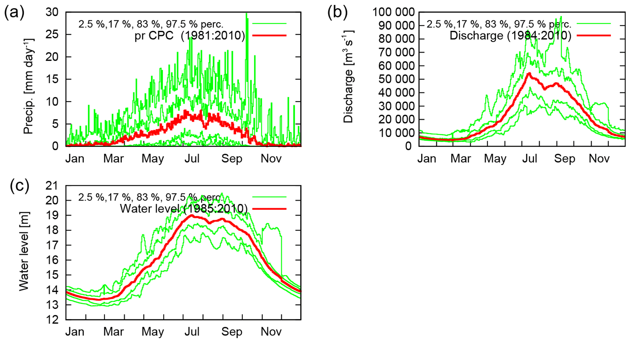
Figure 2Seasonal cycle of (a) precipitation in the Brahmaputra basin for CPC, (b) discharge at Bahadurabad and (c) water level at Bahadurabad. The red line shows the mean value, and green lines show the 2.5, 17, 83 and 97.5 percentiles.
The second gauge-based dataset we use for comparison is the combined Full Data and First Guess Daily 1.0∘ GPCC dataset (1988–now) (Schamm et al., 2013, 2015). As this is a much shorter dataset we expect the signal-to-noise ratio in the trend to be smaller. We only use this dataset to additionally check the observations. The seasonal cycle can be found in the Supplement Fig. S1.
The third dataset is the reanalysis dataset ERA-interim (ERA-int; 1979–now; Dee et al., 2011). Precipitation of this dataset is analysed directly. As well as precipitation, temperature and potential evapotranspiration (calculated with the Penman–Monteith method) are used to drive one of the hydrological models (see Sect. 2.2.4). The seasonal cycle of ERA-int can be found in Fig. S1.
We use discharge and water level data from Bahadurabad. Discharge data are available for the years 1984–2017, and water level data are available for the years 1985–2017 (source: BWDB). For both datasets the seasonal cycle is shown in Fig. 2b, c. Additionally, we have a discharge dataset for the years 1956–2006 (source: BWDB). As the rating between water level, velocity and discharge is not exactly the same in the two discharge datasets, we consider simply merging the datasets not to be appropriate. The 1984–2017 dataset is used in the analyses, but results are compared to calculations with the 1956–2006 dataset and merged datasets.
2.2 Model descriptions
First the global circulation model and regional model that are used for the analysis of precipitation are listed, including a short description of the model runs. Next a list of hydrological models used in this study is given. Further details of the models, including validation and calibration of the hydrological models, are described in the Supplement.
2.2.1 Precipitation
EC-Earth 2.3
We use three different ensembles of the coupled atmosphere–ocean general circulation model EC-Earth 2.3 (Hazeleger et al., 2012) at T159 (∼150 km). The first one is a transient model experiment, consisting of 16 ensemble members covering 1861–2100 (here we use up to 2017), which are based on the historical CMIP5 protocol until 2005 and are based on the RCP8.5 scenario (Taylor et al., 2012) from 2006 onwards. The other two EC-Earth 2.3 experiments are two time-slice experiments based on the 16-member transient model experiment above. Two experimental periods are selected in which the model global mean surface temperature (GMST) is as observed in 2011–2015 (“present-day” experiment) and the pre-industrial (1851–1899) +2 ∘C warming experiment (“2 ∘C warming” experiment).
weather@home
In addition to the EC-Earth 2.3 experiments, large ensembles of climate model simulations are created using the distributed computing weather@home modelling framework (Guillod et al., 2017; Massey et al., 2014) based on Hadley Centre models. Table 1 describes the experiments used in this study, which are grouped into three sets: (i) ensembles for the historical period 1986–2015, (ii) ensembles for 2017 and (iii) ensembles for assessing possible changes in the future.
See the Supplement for a more detailed description of these runs.
Mitchell et al., 2017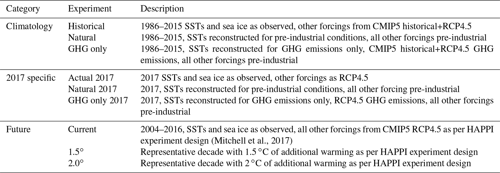
2.2.2 Discharge
PCR-GLOBWB 2
The global hydrological model PCR-GLOBWB 2 (Sutanudjaja et al., 2018) was selected because of its ability to simulate the hydrological cycle, including reservoir operations and human–water interactions at continental and global scales. It resolves the water balance at the surface by using precipitation, temperature and potential evaporation inputs from meteorological observations or climate models. We used PCR-GLOBWB to conduct several river discharge simulations, First we used observational data as input to check the performance of the model. Next we used the EC-Earth transient and two time-slice experiments as input to generate a large ensemble.
SWAT
Second, we use the SWAT, which is a commonly used hydrological model for investigating climate change impacts on water resources at regional scales (Gassman et al., 2014). This model has already been used to simulate impacts of climate change on the flows of the Brahmaputra River (Mohammed et al., 2017, 2018). The water balance equation used in SWAT consists of daily precipitation, runoff, evapotranspiration, percolation and return flow. The SWAT model was used in this study to simulate flows by taking inputs from both the transient and time-slice EC-Earth experiments and weather@home experiments, using daily maximum and minimum temperatures and precipitation.
LISFLOOD
The third hydrological model we use is LISFLOOD. This is a fully distributed and semi-physically based model initially developed by the Joint Research Centre (JRC) of the European Commission in 1997. It was subsequently updated to forecast floods and analyse impacts of climate and land-use change (Burek et al., 2013). It has been used for operational flood forecasts as part of the European Flood Awareness System (EFAS) since 2012 (https://www.efas.eu/en/about, last access: 2 May 2018). The LISFLOOD model was used in this study to simulate the river flow of the Brahmaputra River at the Bahadurabad gauging station with input data from the weather@home model.
River flow model
The fourth and final hydrological model used in the analysis is a fully distributed river flow model (RFM) that estimates the streamflow by discrete approximation of the one-dimensional kinematic wave equation (Dadson et al., 2011). The RFM was used in this study to simulate the river flow of the Brahmaputra River at the Bahadurabad gauging station with input data from the weather@home model.
2.3 Statistical methods
We use a class-based event definition, i.e. we consider all events that are as extreme or more extreme than the observed event on a one-dimensional scale, in this case 10-day averaged precipitation averaged over the Brahmaputra basin or daily runoff at Bahadurabad.
The first step in an attribution analysis is trend detection: fitting the observations to a non-stationary statistical model to look for a trend outside the range of deviations expected by natural variability. In this case we study the trends of extreme high-precipitation and river discharge values. In extreme value analysis, the generalized extreme value (GEV) distribution (Coles, 2001) is often used to fit and model the tail of the empirical distribution for this type of event, the maximum daily or 10-daily value over the monsoon season. The shape parameter ξ determines the tail behaviour, and negative indicates light tail behaviour while positive indicates heavy tail behaviour. When ξ=0, the distribution simplifies to the Gumbel distribution. Global warming is factored in by allowing the GEV fit to be a function of the (low-pass filtered) GMST. In the case of precipitation and discharge extremes, it is assumed that the scale in parameter σ (the standard deviation) scales with the position parameter μ (the mean) of the GEV fit. This assumption is also known as the index flood assumption (Hanel et al., 2009) and is commonly applied in hydrology to restrain the number of fit parameters. It can be checked in the model experiments where there are enough data to fit both μ and σ independently. These parameters are scaled up or down with the GMST using an exponential dependency similar to Clausius–Clapeyron (CC) scaling: , with T as the smoothed global mean temperature and α as the trend that is fitted together with μ0 and σ0. The shape parameter ξ is assumed to be constant. 95 % confidence intervals are estimated using a 1000-member non-parametric bootstrap. This approach has been used in several previous attribution studies (e.g. van Oldenborgh et al., 2016; van der Wiel et al., 2017; Otto et al., 2018). This fit also gives the return periods of the observed event.
The scaling is taken to be an exponential function of the smoothed global mean temperature. This exponential dependence can clearly be seen in the scaling of daily precipitation extremes with local daily temperature in regions with enough moisture availability (Allen and Ingram, 2002; Lenderink and van Meijgaard, 2008). It is also expected on theoretical grounds through the first-order dependence of the maximum moisture content on temperature in the Clausius–Clapeyron relations of about 7 % K−1, which gives rise to an exponential form. Note that we fit the strength of the connection, which is often different from CC scaling. As it is not clear what the relevant local temperature is, but local temperature usually scales linearly with the global mean temperature, we chose the GMST.
The second step in an attribution analysis is the attribution of the detected trend to global warming, natural variability or other factors, such as changes in aerosol concentration or the El Niño–Southern Oscillation; this requires comparing model simulations with and without anthropogenic forcing. There are two approaches. The first is to run two ensembles: one with current conditions and one with conditions as they would have been without anthropogenic emissions. The number of events above the threshold is compared between the two ensembles. In the second approach, we approximate the counterfactual climate by the climate of the late 19th century and fit the same non-stationary GEV that was described above to the model data. The distribution is evaluated for a GMST in the past and the current GMST. These two approaches have been used before for studies of extreme precipitation (e.g. Schaller et al., 2014; van Oldenborgh et al., 2016; van der Wiel et al., 2017; van Oldenborgh et al., 2017). We checked that year-on-year autocorrelations of RX10day (maximum 10-day precipitation amount) are negligible, so serial autocorrelations are not a problem in this analysis.
As a third step, we calculate the risk ratio (RR) or change in probability for different time intervals. These include for instance the difference between the present day and 1979, or between present-day and pre-industrial times. For observations we calculate risk ratios with respect to the beginning of the dataset. If possible, we additionally transform these into risk ratios with respect to pre-industrial conditions, in this case set to be the year 1900, such that we can compare this with model runs for pre-industrial settings. For this transformation we assume that the RR depends exponentially on the covariate, in this case the global mean temperature change. For instance if we find that the probability doubles for 0.5 ∘C warming, we assume that first ordering it would cause it to double again for 1 ∘C warming. With future model runs we can also calculate risk ratios between the +2 ∘C climate and the climate now.
A last step in the analysis is the synthesis of the results into a single attribution statement. Though the method for evaluating risk ratios using a transient model or observations is different from that using ensemble time-slice experiments that are explicitly designed to simulate a +2.0 ∘C world, we are able to give an average value for all observations and models combined, and we assume that this gives a good first-order estimate of the overall risk ratio.
The differences among the RRs of these ensembles and the observations are due to natural variability, different framings and model spread. The relative contribution of random natural variability can be estimated from a comparison of the uncertainty derived from each fit with the spread of the different estimates of the RR from observations and models. We do this by computing a χ2∕dof, with the number of degrees of freedom (dof) being one less than the number of fits. If this is roughly equal to 1, the variability is compatible with only the natural variability that determines the uncertainty on each separate model estimate of the RR. If it is much larger than 1, the systematic differences between the framings and models contribute significantly.
We choose to use a weighted average, with the weights being the inverse uncertainty squared for each RR (models and observations). The uncertainties are approximated by symmetric errors on log (RR) and added in quadrature (). If there is a significant contribution of χ2 due to model spread, this has to be propagated to the final result, and the final uncertainty is larger than the spread due to natural variability. In this case we choose to give all models equal weight. The method described here was also used in Eden et al. (2016) and Philip et al. (2018).
3.1 Precipitation
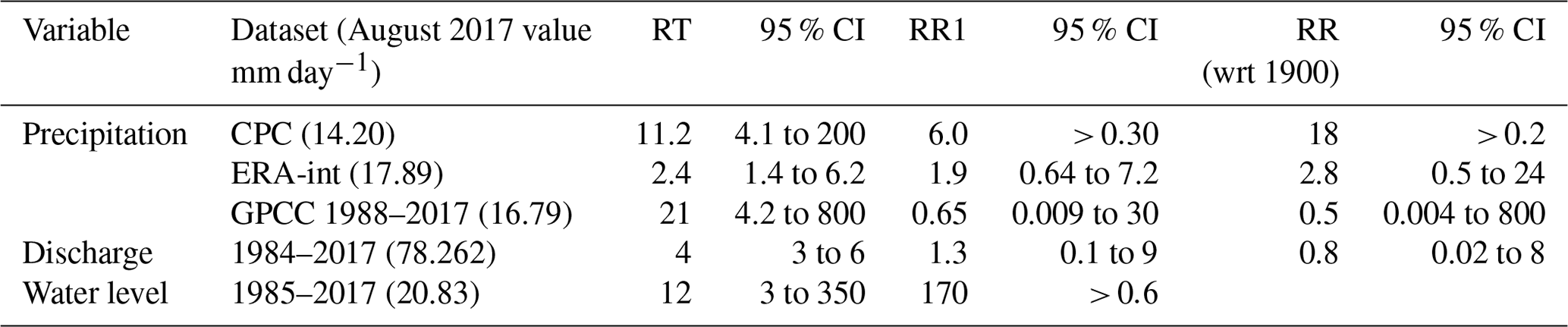
Figure 3a shows the time series of CPC precipitation averaged over the Brahmaputra basin for 90 days ending on 2 September 2017. The 10-day average at the beginning of July is slightly higher than the 10-day average beginning of August, 14.38 versus 14.20 mm. As we are interested in the August flooding event, we take the precipitation value from the August event, which has a maximum on 5–14 August (see Fig. 3c). The 10-day average annual maximum precipitation is fitted to a GEV distribution. The return period plots show that the distribution can be described by a GEV by overlaying the data points and fit for the present and a past climate (Fig. 3d). The return period calculated from this fit is 11 years (95 % CI – confidence interval, 4 to 200 years) for the current climate. There is a positive trend with a risk ratio with respect to 1979 of a factor of 6 (>0.3), although the trend is not significant at p<0.05 when two-sided (the uncertainty range includes 1).
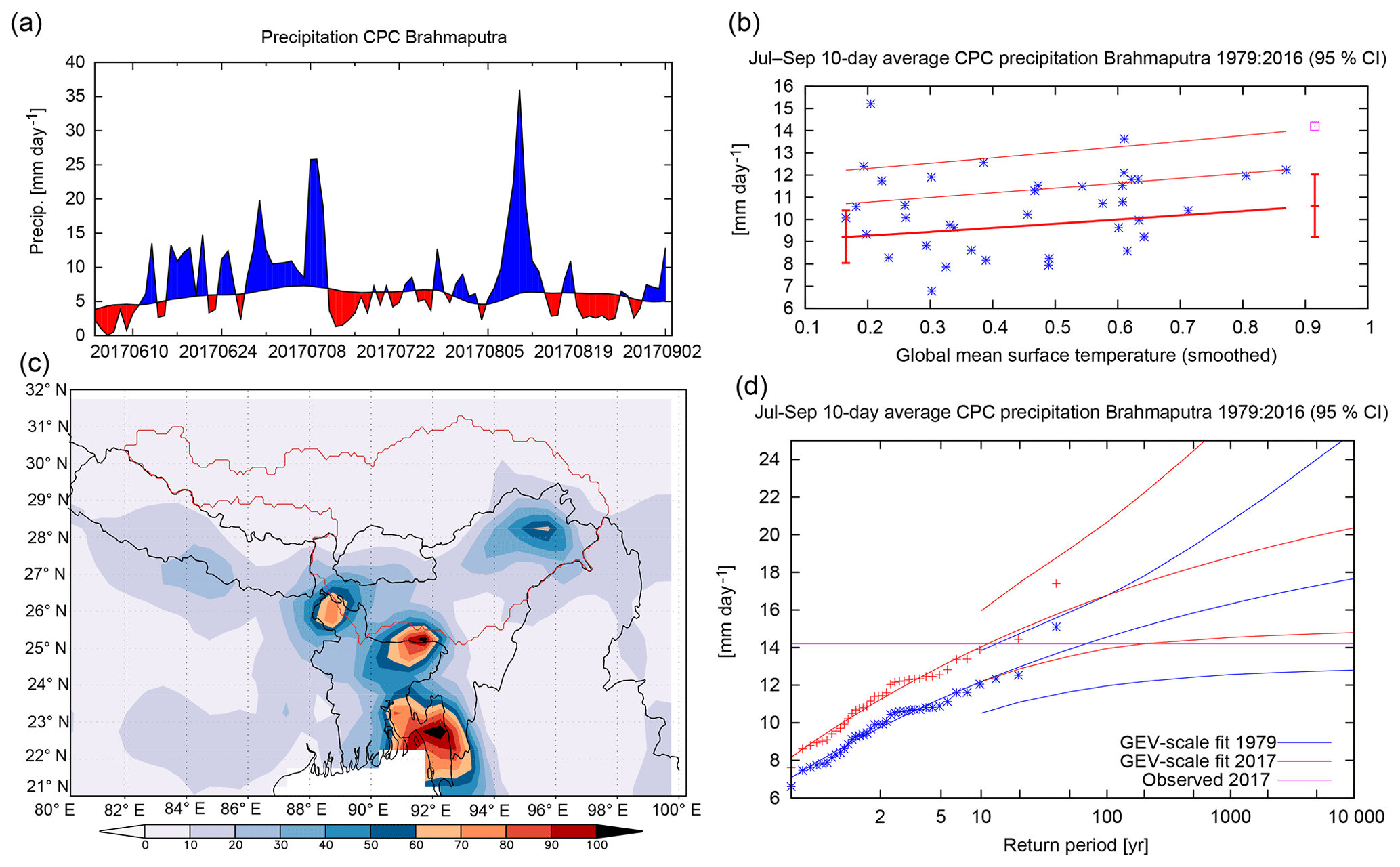
Figure 3CPC data (a, c) and analysis of the highest observed 10-day mean rainfall in the Brahmaputra basin in July–September (b, d). (a) Time series of precipitation averaged over the Brahmaputra basin; blue is more than average, and red is less than average. (b) The location parameter μ (thick line), μ+σ and μ+2σ (thin lines) of the GEV fit of the 10-day averaged data. The vertical bars indicate the 95 % confidence interval on the location parameter μ at the two reference years, 2017 and 1950. The purple square denotes the value of 2017 (not included in the fit). (c) The 10-day averaged precipitation over the Brahmaputra basin. Dark red means heavy precipitation. In red are the contours of the Brahmaputra basin. (d) The GEV fit of the 10-day averaged data in 2017 (red lines) and 1950 (blue lines). The observations are drawn twice, scaled up with the trend (smoothed global mean temperature) to 2017 and scaled down to 1950. The purple line shows the observed value in 2017.
A similar approach to the one used for CPC data is applied to ERA-int data. In this dataset the July 2017 10-day average was also just slightly higher than the August 2017 10-day average. The return period for the August event with a value of 17.9 mm day−1 was 2 years (95 % CI, 1 to 6 years) in the current climate. This dataset also shows a non-significant positive trend with a risk ratio of 1.9 (0.6 to 7), i.e. doubling the probability of an event like this or higher.
Finally, the shorter GPCC dataset gives similar results as well. Risk ratios are given with respect to 1979 in order to compare this with the other datasets. The August 2017 10-day average is slightly higher than the July 10-day average. The return period is about 20 years (95 % CI, 4 to 800 years). The risk ratio is not significantly different from 1.
The results of return periods and risk ratios based on observations can be found in Table 2. For analyses with models we use the return period from the CPC dataset of 11 years for this event, as based on local experience we think that this is the best estimate. Due to the shape parameter being close to zero the risk ratio will not have a strong dependence on this choice; for a Gumbel distribution it is independent of the return time.
Table 2Return periods and risk ratios for observations of precipitation, discharge and water level. The column RR1 gives results wrt 1979 (precipitation), 1984 (discharge) and 1985 (water level). The column RR (wrt 1900) scales the results to the pre-industrial period.
3.2 Discharge
The highest discharge in 2017 was reached on 16 August, with a value of about 78 000 m3 s−1. This was clearly higher than any value in July in the same year, as opposed to the precipitation values discussed above. There have been several years in which the discharge was higher than in 2017, including the years 1998 and 1988, which are the two maximum values in the discharge record. The return period is calculated from the discharge dataset since this is our best observational estimate. However it is worth noting that there is a large uncertainty in the accuracy of the discharge measurements from 2012 onwards. We check if the results are robust by comparing the outcomes from the different datasets.
We fitted the discharge time series of Bahadurabad to a GEV distribution. In this distribution we see no trend (95 % CI with respect to – wrt – 1900 is 0.1 to 40; see Fig. 4). Therefore we calculate the return period assuming no trend. This results in a return period of the August 2017 event of 4 years (95 % CI, 3 to 6 years). A cross-check with the 1956–2006 dataset or merging the two discharge datasets gives similar results.
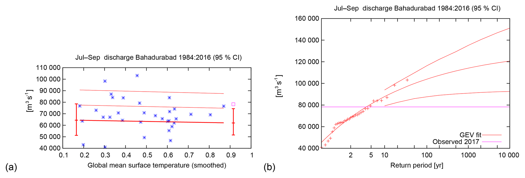
Figure 4Analysis of the highest observed daily discharge at Bahadurabad in July–September. (a) The location parameter μ (thick line), μ+σ and μ+2σ (thin lines) of the GEV fit of the discharge data. The vertical bars indicate the 95 % confidence interval on the location parameter μ at the two reference years, 2017 and 1984. The purple square denotes the value of 2017 (not included in the fit). (b) The GEV fit of the discharge data, assuming no trend. The purple line shows the observed value in 2017.
3.3 Water level
Although we only have the water level available in observations and not for models, we still analyse the observational water level time series from Bahadurabad. The highest value in 2017 was on 16 August, with a value of 20.83 m. This is 1.33 m higher than the dangerous level of 19.50 m. In contrast to the discharge this was a record level since the beginning of the dataset (1985). It should be noted that the water level is also influenced by factors other than climate change, for instance a raising of the river bed by sedimentation and obstruction of the river channel by man-made constructions. See Sect. 6 for a more detailed discussion on the disentangling of geomorphological changes and climate change.
Under the same assumption as that for precipitation and discharge in which water level scales with GMST, the return period in the current climate is estimated to be 12 years (95 % CI, 3 to 350 years; see Fig. 5b). However, although the risk ratio between 2017 and 1985 is as large as 170, this is only non-significant with a lower bound of 0.6. This is probably due to the relatively short length of the dataset. In addition, we calculate a return period assuming no trend (see Fig. 5c). This gives a return period of about 80 years (>25 years, 95 % CI). This agrees with the estimates from BWDB.

Figure 5Analysis of the highest observed daily water level at Bahadurabad in July–September. (a) The location parameter μ (thick line), μ+σ and μ+2σ (thin lines) of the GEV fit of the discharge data. The vertical bars indicate the 95 % confidence interval on the location parameter μ at the two reference years, 2017 and 1985. The purple square denotes the value of 2017 (not included in the fit). (b) The GEV fit of the water level data in 2017 (red lines) and 1985 (blue lines), assuming a trend. The observations are drawn twice, scaled up with the trend (smoothed global mean temperature) to 2017 and scaled down to 1985. (c) The GEV fit of the same discharge data assuming no trend. The purple line in (b) and (c) shows the observed value in 2017.
4.1 Precipitation
In this section we present model validation and analysis results for the precipitation experiments, first for EC-Earth and then for weather@home.
For validation of the EC-Earth 2.3 model we use the years in the transient runs that correspond to the observational years 1979–2017. In the model, as expected, most precipitation falls in the months JJA, with a peak in July, like in observations, though the increase in precipitation is slightly stronger in June than it is in observations (Fig. S1). As it is assumed that the scale parameter σ scales with the position parameter μ of the GEV fit, we check whether the dispersion parameter σ∕μ and the shape parameter in this model are similar to those calculated from observations. The parameters of the GEV distribution that is fitted from the precipitation of these model years correspond well to the same parameters for CPC data.
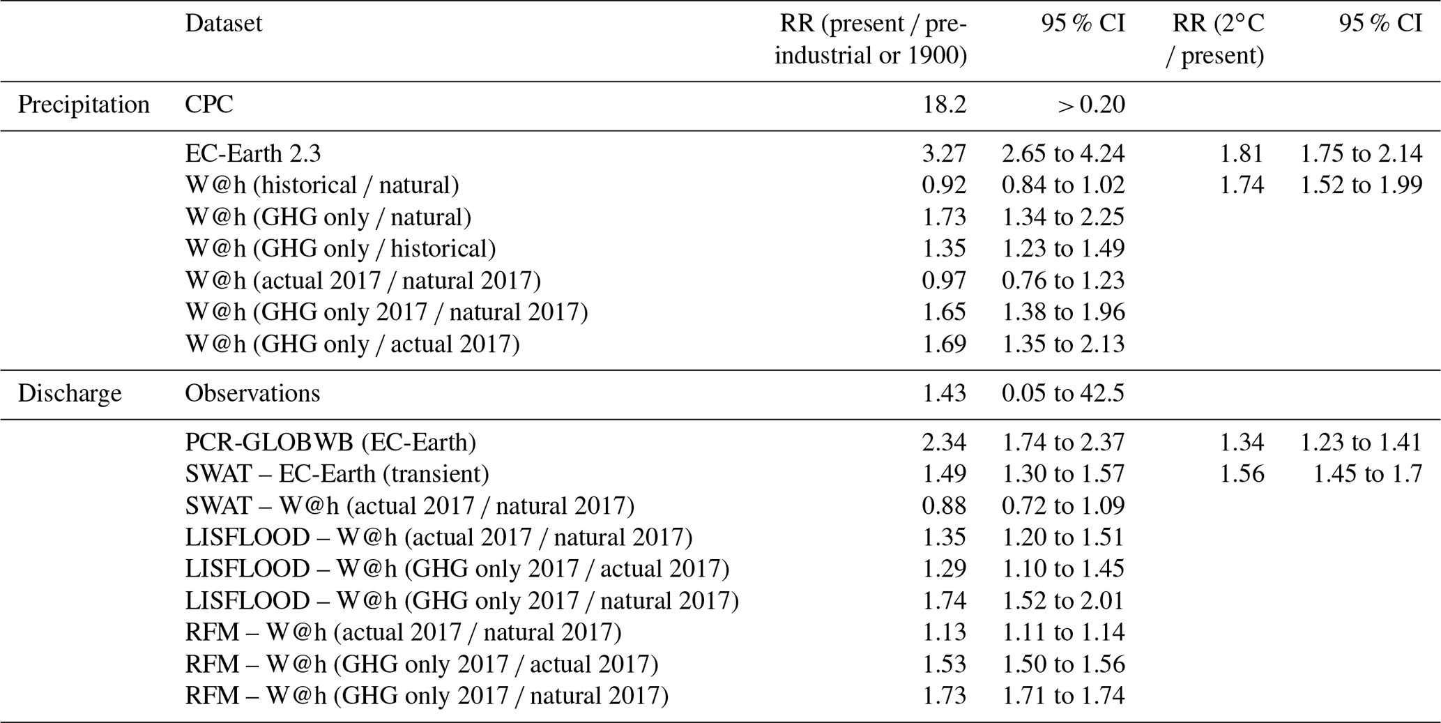
The risk ratio of precipitation is calculated in the same way as that for observations, using the data period 1880–2017 such that we can use the same years for the EC-Earth runs and the PCR-GLOBWB and SWAT runs with EC-Earth input (see Fig. 6). The threshold is chosen such that the return period in the current climate is similar to the observed return period when using the same years. The risk ratio between 2017 and pre-industrial conditions is 3.3 (95 % CI, 2.7 to 4.2) in these transient runs. This corresponds to an increase in intensity for the same return period of 10 % (95 % CI, 9 % to 11 %). For the future (figures not shown) we calculate return periods from the present and future distributions separately, again following the same statistical method as that for observations but with two separate GEV fits that do not depend on the GMST. The risk ratio between a 2 ∘C climate and the present climate follows from this, with a value of 1.8 (95 % CI, 1.7 to 2.1). We thus conclude that in the EC-Earth 2.3 model there is a significant positive trend in the magnitude of precipitation events such as the one in August 2017, both in the past (pre-industrial times up until now) and in the future.

Figure 6Analysis of the highest 10-day average precipitation in July–September in the EC-Earth model in the years 1880–2017. (a) The location parameter μ (thick line), μ+σ and μ+2σ (thin lines) of the GEV fit of the discharge data. The vertical bars indicate the 95 % confidence interval on the location parameter μ at the two reference years 2017 and 1934. (b) the GEV fit of the precipitation data in 2017 (red lines) and 1934 (blue lines), assuming a trend. The data are drawn twice, scaled up with the trend (smoothed global mean model temperature) to 2017 and scaled down to 1934. (c) GEV fits for the present day (PD, red) and +2 ∘C world (2C, yellow) simulations. The purple lines in (b) and (c) show the threshold value for which the risk ratio is calculated.
For weather@home, we compare the annual cycle of 10-day running mean precipitation (see Fig. S2) and its spatial pattern in the Brahmaputra basin from historical simulations with CPC and GPCC observational records. As has also been seen in other regions of Bangladesh (Rimi et al., 2019a), weather@home rainfall is too intense in the pre-monsoon season but lies within observational uncertainty during the monsoon season itself. Also the variability of 10-day model precipitation is under-represented by the model for the monsoon season. During the monsoon season the spatial pattern and magnitude of weather@home output agrees well with GPCC and CPC observations (not shown).
Figure 7 shows the return periods of the maximum 10-day precipitation during JAS from the weather@home simulations, see also Table 3. The threshold used in this analysis is defined by taking the magnitude from the historical simulation corresponding to the return period derived from the CPC observational dataset.
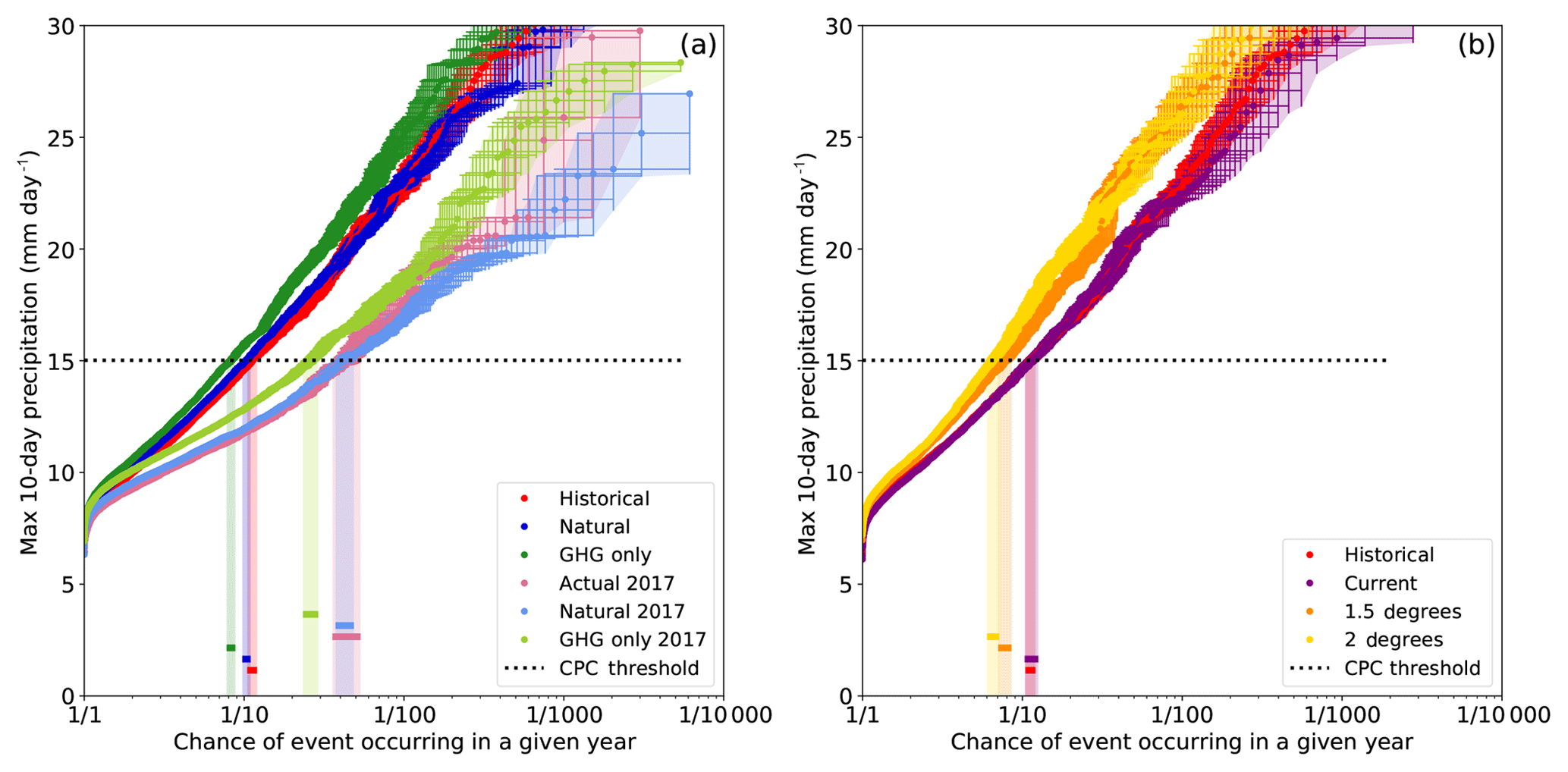
Figure 7Return times of the maximum 10-day precipitation from weather@home simulations. (a) shows results from the historical, natural, GHG-only and actual 2017, natural 2017, and GHG-only 2017 simulations, and (b) shows the historical, current, 1.5 and 2∘ simulations. Black horizontal lines represent the threshold values derived from the CPC observations. Shaded coloured vertical boxes with solid horizontal lines represent the uncertainty in the return period for the CPC threshold.
Figure 7a shows the results for the historical and 2017-specific experiments, which we use to analyse how probabilities may have changed in the period from pre-industrial times up until now. There is no statistically significant difference between the historical and natural simulations, with a risk ratio of 0.92 (0.84to1.02).
The difference in return periods between the historical and actual 2017 experiments gives an indication of the influence of the natural variability of the sea surface temperature (SST) pattern in the precipitation in this region. The historical ensemble is driven by 30 years of differing SST patterns containing different patterns of natural variability such as the El Niño–Southern Oscillation, whereas actual 2017 uses only the observed 2017 Operational Sea Surface Temperature and Sea Ice Analysis (OSTIA) SSTs. The SST pattern in 2017 (actual 2017) made extreme precipitation events less likely than the climatological mean (historical) with a risk ratio of 0.25 (95 % CI, 0.2 to 0.31). Within the set of simulations conditioned on 2017 SSTs, the negligible anthropogenic influence found in the full range SST set is confirmed; the actual 2017 and natural 2017 ensembles also do not show a statistically significant difference and have a risk ratio of 0.97 (95 % CI, 0.76 to 1.23), indicating that, if anything, high-precipitation events similar to the amplitude observed are more prevalent in our model in the natural ensemble, whether or not conditioned on 2017 SST conditions.
To understand this result more fully it is useful to look at the “GHG-only” simulations in Fig. 7a (compare GHG-only with historical simulations and GHG-only 2017 with actual 2017 simulations). The GHG-only simulations show that increased GHG emissions have increased the likelihood of this kind of event (relative to the natural simulations) but that when the sulfate aerosol emissions are taken into account (in the historical and actual 2017 simulations), we find a counterbalancing effect that acts to reduce rainfall, hence reducing the risk for severe flooding. This effect has also been noted by van Oldenborgh et al. (2016); Rimi et al. (2018b). Within the weather@home model sulfate emissions are included, although emissions due to other important aerosols such as black carbon, which can counteract sulfate effects, are not represented. The aerosol effect in HadRM3P is therefore potentially overestimated. The results highlight the non-linear change in risk over time as a function of anthropogenic aerosol emissions. EC-Earth follows the historical+RCP8.5 protocol for aerosols and includes both sulfate emissions and black and organic carbon. It does not include any indirect aerosol effects. The differences in aerosol representation and model handling of aerosols, as well as the influence of the experimental configuration on aerosol concentration, between EC-Earth and weather@home may account for the difference in risk ratios for the past climate period (pre-industrial times up until now) between the two models, whereas the change in risk of future climate scenarios show good agreement.
Figure 7b shows return periods from the historical, current, natural, 1.5 and 2.0∘ simulations, which we use to analyse how probabilities may change in the future with respect to now. The current and historical ensembles are very similar as expected as both are forcing simulations of differing (but overlapping) lengths. Under 1.5 and 2 ∘C of additional warming, high precipitation within the region is set to increase with risk ratios (compared to current simulation) derived using the CPC observational threshold of 1.46 (95 % CI, 1.27 to 1.69) and 1.74 (95 % CI, 1.52 to 1.99) respectively. In both cases the ERA-int (GPCC) threshold risk ratio is smaller (larger) than the CPC threshold risk ratio (not shown), but with overlapping uncertainty bounds with CPC. For 2 ∘C of warming these risk ratios show good agreement with the EC-Earth values.
Table 3Risk ratios for precipitation and discharge for models and observations for both present to pre-industrial times or 1900 and a 2 ∘C climate to present. 95 % confidence intervals are given as well.
4.2 Discharge
In this section we present model validation and results of the discharge simulations, first for the model PCR-GLOBWB and then for SWAT, LISFLOOD and the RFM.
The runs with the PCR-GLOBWB model are treated in the same way as the EC-Earth runs. The experiment in which the PCR-GLOBWB model is driven by CPC precipitation and ERA temperature and evapotranspiration shows a strong trend in discharge, which was not seen in the discharge observations. The GEV-fit parameters encompass the best estimate from observations when fitted with a trend. However the large discharge events of 1988 and 1998 are not captured in this run (not shown).
The experiment with ERA input, in contrast, shows no trend but clearly shows the strong discharge events of 1988 and 1998 (not shown). The best estimate of the GEV-fit parameter is outside the error margins of the GEV-fit parameters of observations; however, the error margins overlap.
These two model runs show that the PCR-GLOBWB model is able to capture historical flood events, but the magnitude of these events is dependent on the meteorological input data. Furthermore, we find that the statistical properties are a fair representation of the statistical properties of observed discharge.
We perform an additional validation of the transient PCR-GLOBWB run with EC-Earth 2.3 input over the years corresponding to years with observed discharge. With this input the modelled discharge peaks in August but is also high in July and September. We thus use the same months JAS as in observations for further analysis. Different from the observed distribution, the shape parameter ξ is positive, showing higher discharge values in the tail. This is not a problem for this analysis, as the return period of about 4 years that we are interested in is not in the tail of the distribution. When comparing the error margins of the ratio σ∕μ with observed statistics we note that the model variability is too large compared to the model mean. This is not the ideal situation, and we note in the discussion how this model bias affects the analysis.
Using the transient model runs, the risk ratio of discharge is calculated in the same way as that for observations, using all data between 1880–2017. The risk ratio between 2017 and pre-industrial times is 2.3 (95 % CI, 1.7 to 2.4; see Fig. 8). For the future we calculate return periods from the present and future distributions separately, following the same statistical method as that for precipitation in the EC-Earth 2.3 present and future experiments. The risk ratio between a 2 ∘C climate and the present follows from this, with a value of 1.3 (95 % CI, 1.2 to 1.4). We thus conclude that in the PCR-GLOBWB model driven by EC-Earth output there is a positive trend in discharge events like the one in August 2017 in both the historical period (pre-industrial times to 2017) and the future period (from current conditions to a +2 ∘C world).
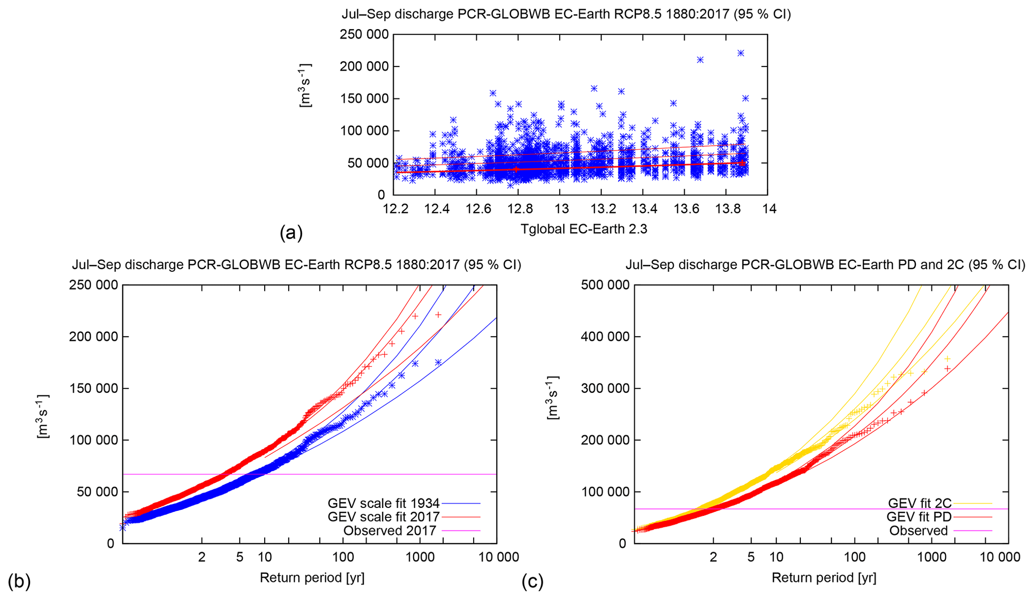
Figure 8Analysis of the highest discharge at Bahadurabad in July–September in the PCR-GLOBWB model in the years 1920–2017. (a) The location parameter μ (thick line), μ+σ and μ+2σ (thin lines) of the GEV fit of the discharge data. The vertical bars indicate the 95 % confidence interval on the location parameter μ at the two reference years 2017 and 1934. (b) The GEV fit of the discharge data in 2017 (red lines) and 1934 (blue lines), assuming a trend. The observations are drawn twice, scaled up with the trend (smoothed global mean model temperature) to 2017 and scaled down to 1934. (c) GEV fits for the present day (PD, red) and +2 ∘C world (2C, yellow) simulations. The purple horizontal lines in (b) and (c) show the threshold value for which the risk ratio is calculated.
The SWAT model calibrated with EC-Earth meteorological data tends to underestimate flows in almost all months of the year (see Fig. S3 in the Supplement). The SWAT model calibrated with weather@home meteorological data, in contrast, tends to underestimate flows in the monsoon months while overestimating flows in the remaining months. Therefore in both cases, flows in our months of interest (JAS) are always slightly underestimated, but the magnitudes of error appear limited enough for the models to be useful in conducting attribution studies. When comparing the error margins of the ratio σ∕μ with observed statistics we note that the model variability is too small compared to the model mean, opposite to what was found for the PCR-GLOBWB model. The shape parameter ξ is of the same order as the one in the observed discharge dataset.
The risk ratios are calculated from return period plots for both the EC-Earth runs (see Fig. 9) and the weather@home runs (see Fig. 10). Using the SWAT model runs with EC-Earth transient data, we see that the discharge shows some decadal variability. The trend in the data therefore depends more strongly on the years used. For consistency we use the same years as in the analyses of EC-Earth and PCR-GLOBWB data (1880–2017), and we note that the error margins do not capture this variability and are underestimated. The risk ratio of discharge between 2017 and pre-industrial times is found to be 1.5 (95 % CI, 1.3 to 1.6). The risk ratio between a 2 ∘C climate and the current climate is 1.56 (95 % CI, 1.45 to 1.70). Using the SWAT model runs with weather@home actual 2017 and natural 2017 data, the risk ratio between the actual 2017 and natural 2017 scenario is 0.88 (95 % CI, 0.72 to 1.09).
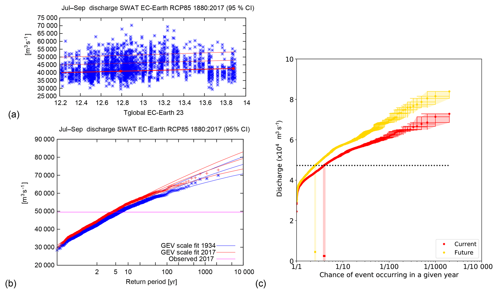
Figure 9Analysis of the highest discharge at Bahadurabad in July–September in the SWAT flows for EC-Earth. (a) the location parameter μ (thick line), μ+σ and μ+2σ (thin lines) of the GEV fit of the discharge data. The vertical bars indicate the 95 % confidence interval on the location parameter μ at the two reference years, 2017 and 1934. (b) the GEV fit of the discharge data in 2017 (red lines) and 1934 (blue lines), assuming a trend. The observations are drawn twice, scaled up with the trend (smoothed global mean model temperature) to 2017 and scaled down to 1934. (c) current and future simulations. The purple horizontal line in (b) and dotted line in (c) show the threshold value for which the risk ratio is calculated.
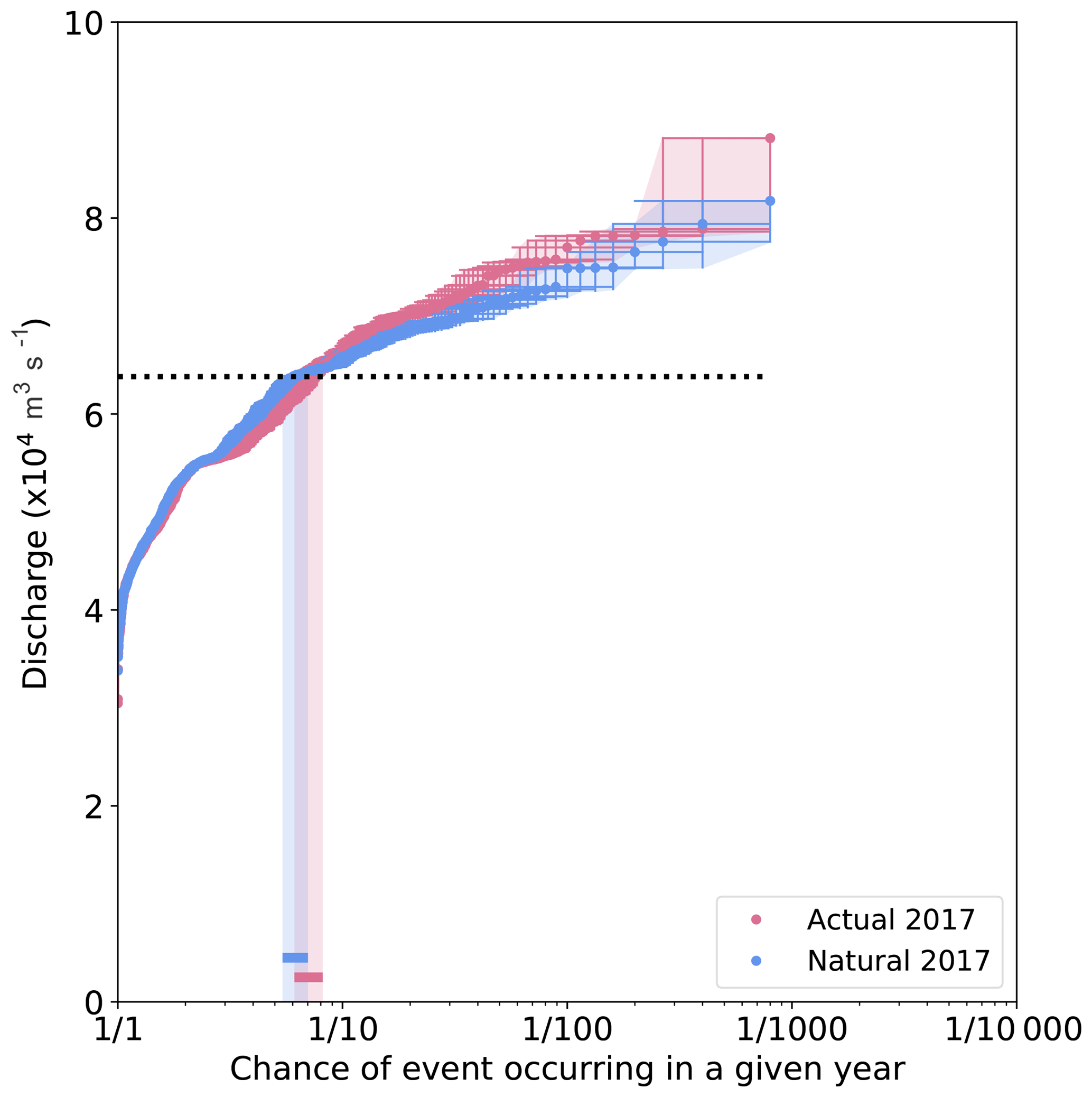
Figure 10Return period plots for SWAT flows with weather@home data for the actual 2017 and natural 2017 ensembles.
Calibration and validation graphs for LISFLOOD and the RFM are shown in the Supplement. They show that both LISFLOOD and RFM are able to simulate the seasonality of rise in spring and summer flows correctly. Both models underestimate the river discharge in summer, with an underestimation in the simulated discharge by LISFLOOD.
The return period and risk ratio for the LISFLOOD model and RFM estimated from the weather@home actual 2017 and natural 2017 datasets, as well as the results for the GHG-only 2017 runs, are shown in Fig. 11.
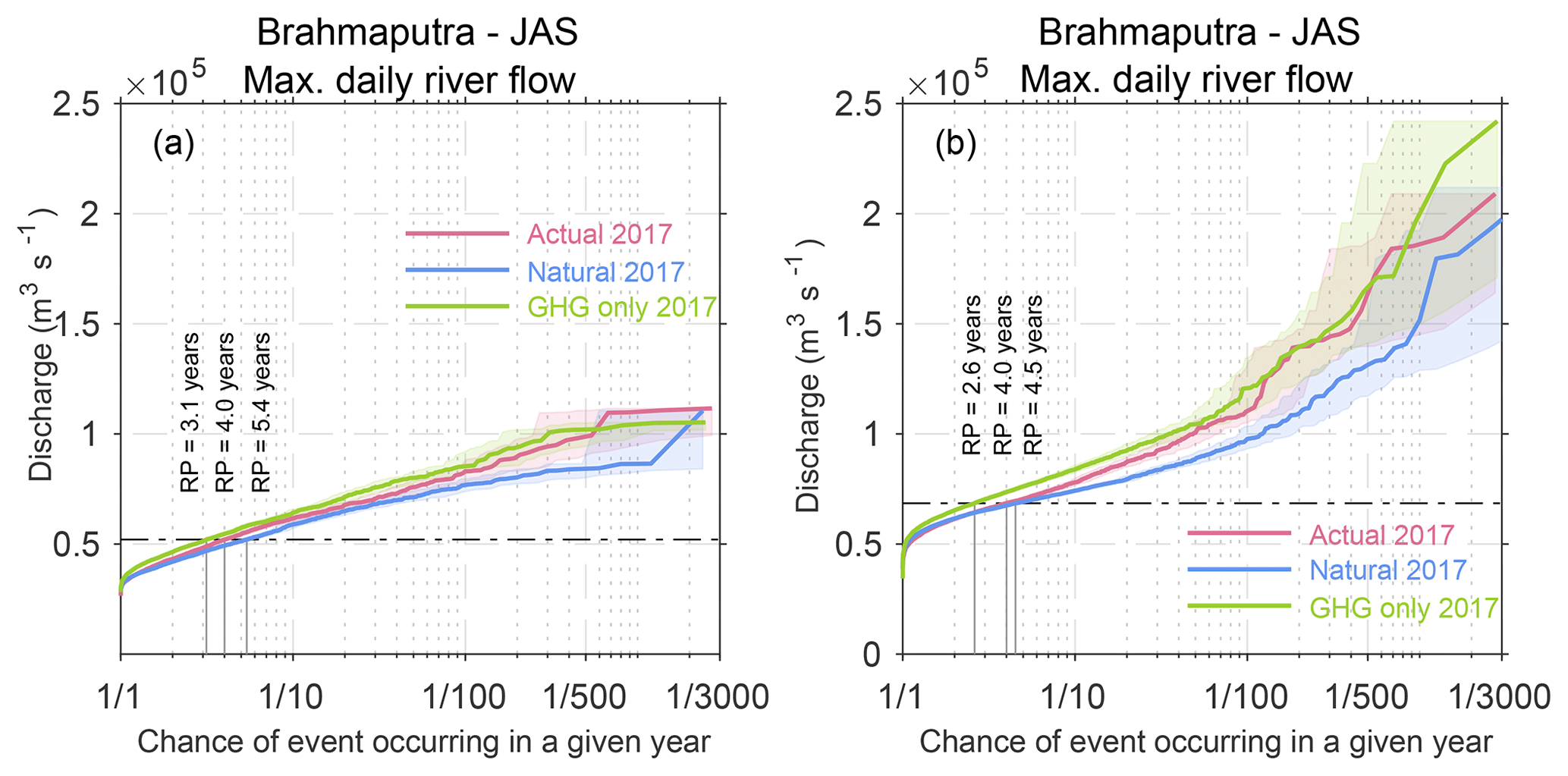
Figure 11River flow return periods simulated by (a) LISFLOOD and (b) RFM using the actual 2017, natural 2017 and GHG-only 2017 scenarios.
The LISFLOOD model shows that a discharge value with a return period of 4 years in the actual scenario would increase to 5.4 years in the natural climate scenario (risk ratio of 1.35 – 95 % CI, 1.20 to 1.51), while it would reduce to 3.1 years in the GHG-only scenario.
The trend is similar in the results simulated by the RFM, however, the discharge value with a return period of 4 years is slightly greater than the value simulated by LISFLOOD. The return period would increase to 4.5 years under natural climate conditions (risk ratio of 1.13 – 95 % CI, 1.11 to 1.14), while it would reduce to 2.6 years in the GHG-only scenario. Note however that from Fig. 11b we see that the risk ratio between the different scenarios for RFM becomes larger for larger return periods (e.g. 10 years) than those studied in this analysis.
The shorter return period in the GHG-only 2017 scenario shows that if sulfate aerosols are removed from the atmosphere (which results in increased precipitation), flooding becomes more frequent. This implies that floods can become more frequent in the region if the air pollution levels are reduced in the future.
The risk ratios for the observed threshold from both LISFLOOD and the RFM of 1.35 (95 % CI, 1.20 to 1.51) and 1.13 (95 % CI, 1.11 to 1.14) respectively are in good agreement even though the simulated river flows by the models are different. The mitigation effect due to the aerosols is also comparable between these two different hydrological models.
In observations the uncertainties in return periods and risk ratios are quite large. This is mainly due to the shorter lengths of the time series, and natural variability dominates. In the models, the signal-to-noise ratio is much larger, resulting in smaller uncertainties in the risk ratios. Here, the model spread dominates the signal. As both natural variability and model spread play a role, we use a weighted average with inflated uncertainty range. We do not synthesize the risk ratios for the future, as we only have two model estimates per variable.
In the synthesis we use all available observational datasets that are analysed in this paper and one experiment per model. For weather@home and all hydrological models that use input from weather@home experiments we use the risk ratios calculated from the actual 2017 and natural 2017 experiments. This gives us a fair opportunity to compare the synthesis of precipitation with the synthesis of discharge.
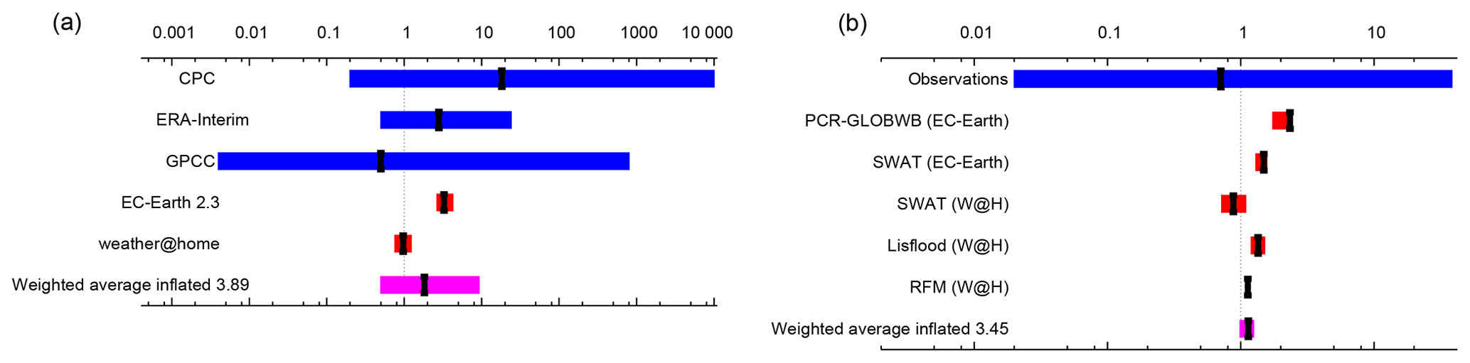
Figure 12Synthesis of the precipitation (a) and discharge (b) results. Dark blue is observations, red is climate model ensembles and the weighted average is shown in purple. The ranges of the models are not compatible with each other, pointing to model uncertainty playing a role over the natural variability. The weighted average has been inflated by factors of 3.89 and 3.45 for precipitation and discharge respectively to account for the model spread.
The synthesis results are shown in Fig. 12. The synthesis of the precipitation analysis results in a risk ratio between 2017 and pre-industrial times of 1.8 (95 % CI, 0.5 to 9.3). Although the best estimate is above 1, the trend is not significant due to the relatively large error margins. The synthesis of the discharge analysis results in a risk ratio between 2017 and pre-industrial times of 1.1 (95 % CI, 1.0 to 1.3). So for discharge the best estimate is only slightly higher than 1, and due to the smaller error margins in the average, this trend is only significant under the assumptions made in this analysis.
In any event-attribution study, tasks to be carried out include the following:
- i.
determining what happened using available observations and defining the event to be studied,
- ii.
determining how rare the event is in current and pre-industrial conditions,
- iii.
using models to attribute any changes in likelihood of similar classes of events.
Here we discuss some of the issues encountered in these steps and the interpretation of our results in the light of uncertainties.
First of all, determining the amount of precipitation falling into the Brahmaputra basin from observations (and thus the appropriate precipitation threshold to define this event) is not trivial. As is common in regions with strong topographic gradients, estimating area-averaged rainfall based on observed rainfall is challenging, as rainfall differences between neighbouring locations can be very large in reality, and the orography, which is only partly resolved by a sparse observational network (or model grid), drives these differences. A large part of the Brahmaputra basin has an elevation of over 2000 m; hence unsurprisingly different precipitation datasets show very different spatial and temporal characteristics. They are all likely to underestimate the precipitation at higher elevations, where few weather stations record data (Immerzeel et al., 2015).
For this analysis we used the CPC dataset to provide a single estimate of the event magnitude (i.e. determine what happened) and to define the return period (i.e. determine the rarity of the event) for use in the other datasets and models. Applying this return period, we used three observational datasets to convey the uncertainty related to observations in the resulting risk ratios. However, for the GPCC dataset, the very limited temporal length of the record leads to an uncertainty estimate that is too high for meaningful inference on the change in risk to be made. The longer records do show an increase in the chance of extreme rainfall, but again uncertainties affect a clear signal detection. The intended future availability of high-resolution reanalyses such as ERA5 that will cover the years 1950 onwards at 30 km resolution will potentially improve trend analyses in high-mountain regions in Asia.
From the hydrological perspective, we defined the event as the maximum daily discharge at Bahadurabad in July–September. In contrast to precipitation data, there is only one official discharge observation series, which does not allow for intercomparison. The determination of flood risk, however, appears to be sensitive to the hydrological variable studied. To obtain an impression of this sensitivity, we checked how discharge compares to the water level as a second measure for the likelihood of flooding. The return period of the measured 2017 discharge peak is indeed lower than the return period of the measured 2017 water level peak. Several factors could have influenced this. First of all, the Brahmaputra is a highly braided river, and during severe flood events water enters the floodplain, making it more difficult to accurately relate water level measurements to discharge estimates. Therefore though the water level records are very accurate, the discharge records are unlikely to be of the same accuracy. Based on the observation of the massive spatial extent of the 2017 floods both in Bangladesh and India, we opine that the observed discharges are likely higher than those recorded.
This opinion is supported by the change in correlation between discharge and water level. The correlation between water level and discharge is 0.88 over the whole time series. However, after 2011 this correlation changes to almost 1, with a tendency toward discharges values that are lower for similar water levels than before this change. This change could be due to recalibration of the relationship between discharge and the water level. We therefore expect that the true return period is between the return period calculated from discharge given above and the return period calculated from the water level. As we do not know the exact influence of the change in measurement method of discharge on the discharge values, we cannot give more precise values.
However it should be noted that ongoing morphological changes can introduce additional variability along the river. For instance, higher water levels with lower discharges may be caused by silting and narrowing of the river. McLean and O'Connor (2013) already showed that, for the years 2006–2011, the relation between discharge and water level changes over time; in 2011 similar discharge values led to higher water levels. This leads to a non-climatic trend in the water level observations.
The disentangling of the influence of climate change and geomorphological changes was beyond the scope of this analysis. On top of qualitatively good observations of the water level, it would require observational data on geomorphological changes, more detailed local hydrological models that can incorporate these and calculate water levels with substantial accuracy, and an additional set of model experiments. In the current analysis we mainly used discharge data and climate model experiments, and from these results it is not possible to conclude whether neglecting geomorphological changes in the models leads to any disagreement with observations given the large uncertainties in the observational analysis.
Climate models, while far from perfect in their representation of reality, are essential for interpreting the results from observations and thereby attributing any observed changes in event frequency to anthropogenic climate change or other factors. Taken at face value, the two climate model simulations of 10-day precipitation maxima in the Brahmaputra basin provide somewhat contradictory results. However, for the weather@home simulations when comparing the natural simulations with GHG-only runs instead of historical simulations, the change in extreme precipitation is significantly positive as well and is therefore more comparable in magnitude to the increase in the two longer observational datasets and EC-Earth simulations. Comparing the GHG-only runs to the historical simulations gives an indication of the impact of aerosol within the weather@home model, which might be slightly overestimated given that black carbon is not included in the models aerosol treatment. Nonetheless, HadRM3P clearly indicates that the increased risk in extreme rainfall due to GHG induced warming has been effectively counterbalanced by aerosol emissions. The EC-Earth model is interpreted as having fewer aerosol effects and hence showing more of the greenhouse-gas-driven increase. Both results are in agreement with the observations due to the large uncertainties in the limited-length observational records.
The counterbalance between the greenhouse-gas and aerosol effects may also be important for clean air policy decisions; as the air is cleaned the already-committed increase in extreme precipitation due to greenhouse gases will be revealed. These results also suggest that the overall signal from long-term climate change, i.e. mainly greenhouse-gas forcing, in the datasets where we cannot separate out the impact of aerosol forcing might be underestimated. The best estimate of the change in risk in extreme rainfall as observed in the Brahmaputra basin in 2017 is therefore likely a rather conservative estimate and hence is of limited use to inform decision-making. In fact, simulations of the near future in both models show a clear increase in the risk of high-precipitation events that lead to flooding in the Brahmaputra.
In extending our multi-method attribution approach to include hydrological modelling, we consequently introduced more degrees of freedom in possible combinations of inputs and models to construct the hydrological response. Time and computational restraints put a limit on the number of combinations that could be explored. We conducted experiments using (i) the same hydrological model (PCR-GLOBWB) run at different resolutions with different input observational and/or modelled meteorological input data, (ii) the same input climate model (weather@home) with different hydrological models, and (iii) the same hydrological model (SWAT) with two different input climate models. Changing the resolution of the PCR-GLOBWB runs with CPC and ERA-int input compared to runs with EC-Earth 2.3 input impacts the dynamics in the hydrological model. In general coarser-resolution simulations respond faster due to the decrease in storage and the shorter connectivity between grid cells. High-resolution models are better able to capture the subsurface and riverine water storage due to their increased heterogeneity (Sutanudjaja et al., 2018). It is therefore more difficult to simulate extreme hydrological events in coarser models (Samaniego et al., 2018). It was beyond the scope of this paper to analyse the differences in detail; however, we use the differences to show the range of possible output within one hydrological model. None of the models or observational datasets are perfect. For instance, in the PCR-GLOBWB model the variability is too high compared to the mean, while RFM and LISFLOOD underestimate the magnitude considerably. This is not the ideal situation however, there is no reason to believe that the order of magnitude of the risk ratios between the current and past climate or between the future and current climate will depend on this very strongly. This is corroborated by the fact that the risk ratios are comparable despite the very different biases.
Despite these strong differences in variables, resolution, simulated processes and input data, the simulated changes in the likelihood of the observed event occurring because of anthropogenic climate change are very comparable. Even when the hydrological models are driven by precipitation from the weather@home simulations the simulated discharge shows a significant increase in likelihood, apart from SWAT, where the change is not significant.
In August 2017, following heavy rains, Bangladesh faced one of their worst river flooding events in recent history, with record high water levels leading to inundation of river basin areas in the northern parts of the country, impacting millions of people who are highly exposed and vulnerable to unusual flooding.
This paper presents an attribution of this precipitation-induced flooding event and, for the first time, extends the multi-method approach of extreme event attribution from a purely meteorological perspective to the more impact-relevant hydrological perspective by employing an ensemble of hydrological models. Firstly, experiments were conducted with three observational datasets and two climate models to estimate changes in extreme precipitation event frequency, in the 10-day Brahmaputra basin average, that have occurred since pre-industrial times. In addition, climate projection experiments were used to indicate if the trends found up until now are likely to continue or become more extreme in the future. The precipitation series were then used in turn as meteorological input for four different hydrological models to estimate the corresponding changes in river discharge. In doing so, a range of possible answers to the attribution question were produced, allowing for comparison between approaches and for the robustness of the attribution results to be assessed.
Specifically, our aims were to (i) determine if precipitation can be used as a measure of the extremity of flooding in the large Brahmaputra basin, or if it is necessary to instead use a hydrological measure such as discharge for the purpose of attributing the flood of August 2017 in Bangladesh, and to (ii) draw conclusions on the attribution of this event, expressed as the change in likelihood of similar or more extreme events, that has occurred since pre-industrial times and which is projected to occur in the future.
From the precipitation perspective, we find that two out of three of the observed series show an increased probability for extreme precipitation like observed in August 2017, but in all three observational datasets the trends are not significant due to the short records. One climate model shows a significant positive influence of anthropogenic climate change, whereas the other simulates a cancellation between the increase due to greenhouse gases and a decrease due to sulfate aerosols. The change in risk of high precipitation that has occurred since pre-industrial times is therefore uncertain. However, both climate models agree that the risk will increase significantly in the future, by more than 1.7, with 2 ∘C of global heating since pre-industrial times.
Considering discharge rather than precipitation, which corresponds more closely with the hydrological impacts, shows only a slightly different result in that only the increase in risk since pre-industrial times to present-day conditions of high discharge synthesized from both observations and models is just significant, whilst the risk of high precipitation is not. The attribution of the change in discharge is therefore somewhat less uncertain than for precipitation, but the 95 % CI still encompasses no change in risk. For the future, these models project a slightly smaller increase in probability of high discharge than of high 10-day precipitation, being more likely by about a factor of 1.5 in a 2 ∘C warmer world.
For large basins in orographically diverse regions with complex hydrology, such as the Brahmaputra, we hypothesized that rainfall, river flow and inundation would not be linearly connected and that precipitation would not be an adequate measure of flood intensity. The initial hydrological conditions play an important role in combination with the occurrence of high intensity precipitation events. We therefore anticipated that small changes in the risk of precipitation would lead to disproportionate changes in flood risk, evidenced in differences in the risk ratios of the event calculated from the two perspectives.
Our synthesis, however, produces the best estimate for the past climate that is greater than 1 and of a similar order of magnitude (between 1 and 2) for both methods and a lower bound on the uncertainty range that is less than or about equal to 1, leading to the conclusion that we cannot confidently confirm a significant anthropogenic influence in changes up until now. Projected changes between current conditions and for a world 2 ∘C warmer than the pre-industrial one were also a similar order of magnitude (between 1 and 2) for 10-day precipitation and discharge, with significant changes found. Thus, in this particular case, studying precipitation alone would have led to the same qualitative conclusion.
Inspecting the individual model outcomes shows that in the study of this particular event, there is an impact of the choice of circulation model used as input for the hydrological model on the amplitude of discharge RRs. Where the EC-Earth model was used, we find a larger positive change in precipitation compared to discharge, but where the weather@home model was used, we find a similar or smaller positive change in precipitation compared to discharge. This highlights the importance of using multiple models in attribution studies, particularly where the climate change signal is not strong.
The use of multiple methods in the attribution of extreme events is the only way to estimate confidence, and hence reliability, in attribution results. As hydrological models are used to simulate impact-relevant variables (such as flood depth) and are in fact used much more for decision-making, it is essential to extend the attribution approach in general to include hydrological models, when possible, for analysis of precipitation-induced flood events. Hydrological models offer further insight into the partitioning of precipitation reaching the ground and thus come closer to the drivers of the impacts observed on people and livelihoods. Climate models, in contrast, allow us to disentangle the potential effects of different atmospheric drivers.
This highlights that only a combination of doing a multi-method attribution analysis of the meteorological drivers with a multi-model approach in hydrological modelling allows for a robust estimate of changing flood hazards under climate change. Therefore we recommend the use of a hydrological variable, such as discharge, for estimating changing flood risk in large basins such as the Brahmaputra, although based on this study, investigating changes in precipitation is also useful, either as an alternative when hydrological models are not available or as an additional measure to confirm qualitative conclusions.
Almost all data are available for download and analysis under https://climexp.knmi.nl/selectfield_att.cgi (last access: 20 July 2018) under section “Bangladesh flooding 2017”, including the GPCC data (Schamm et al., 2013, 2015) used in this study.
The supplement related to this article is available online at: https://doi.org/10.5194/hess-23-1409-2019-supplement.
SP, SS and SFK designed the research. SP, SS and SFK wrote the paper with contributions from all other authors. SP and SFK analysed the observational data, EC-Earth 2.3 data and PCR-GLOBWB data. SS and FELO analysed the weather@home data. HJ and FH provided and analysed the LISFLOOD and RFM data. KM and AKMSI provided and analysed the SWAT data. NW and KvdW provided the PCR-GLOBWB data. KH prepared the weather@home simulations. RHR validated the weather@home data. DCHW managed the weather@home system. AH and KM provided observational water level and discharge data. GJvO supervised the project and contributed analysis tools, and RS and AH contributed with local information.
The authors declare that they have no conflict of interest.
Sarah Sparrow, Hammad Javid, Karsten Haustein, David C. H. Wallom,
Friederike E. L. Otto and A. K. M. Saiful Islam were funded as part of the
EPSRC GCRF Institutional Sponsorship REBuILD project. Karin van der Wiel was funded
as part of the HiWAVES3 project. Niko Wanders acknowledges the funding from
NWO 016.Veni.181.049. This work was partially supported by the EUPHEME
project, which is part of ERA4CS, an ERA-NET initiated by JPI Climate and
co-funded by the European Union (grant 690462). We would like to thank the
Met Office Hadley Centre PRECIS team for their technical and scientific
support for the development and application of weather@Home. We are grateful
to Simon Dadson and Homero Paltan Lopez for sharing the RFM code and for
their help in setting it up for the study area. Finally, we would like to
thank all of the volunteers who have donated their computing time to
climateprediction.net and weather@home.
Edited by: Bob Su
Reviewed by: Vahid Rahimpour Golroudbary
and two anonymous referees
Allen, M. R. and Ingram, W. J.: Constraints on future changes in climate and the hydrologic cycle, Nature, 419, 224–232, https://doi.org/10.1038/nature01092, 2002. a
Burek, P., Knijff van der, J., and Roo de, A.: LISFLOOD, distributed water balance and flood simulation model revised user manual 2013, Publications Office of the European Union, Directorate-General Joint Research Centre, Institute for Environment and Sustainability, https://doi.org/10.2788/24719, 2013. a
CEGIS and SEN authors: Assessing the economic impact of climate change on agriculture, water resources and food security and adaptation measures using seasonal and medium range of forecasts, coordinated by ICIMOD, Nepal, 2013. a
Coles, S.: An Introduction to Statistical Modeling of Extreme Values, Springer Series in Statistics, London, UK, 2001. a
Dadson, S., Bell, V., and Jones, R.: Evaluation of a grid-based river flow model configured for use in a regional climate model, J. Hydrol., 411, 238–250, https://doi.org/10.1016/j.jhydrol.2011.10.002, 2011. a
Dastagir, M. R.: Modeling recent climate change induced extreme events in Bangladesh: A review, Weather and Climate Extremes, 7, 49–60, https://doi.org/10.1016/j.wace.2014.10.003, 2015. a
Dee, D. P., Uppala, S. M., Simmons, A. J., Berrisford, P., Poli, P., Kobayashi, S., Andrae, U., Balmaseda, M. A., Balsamo, G., Bauer, P., Bechtold, P., Beljaars, A. C. M., van de Berg, L., Bidlot, J., Bormann, N., Delsol, C., Dragani, R., Fuentes, M., Geer, A. J., Haimberger, L., Healy, S. B., Hersbach, H., Hólm, E. V., Isaksen, L., Kållberg, P., Köhler, M., Matricardi, M., McNally, A. P., Monge-Sanz, B. M., Morcrette, J.-J., Park, B.-K., Peubey, C., de Rosnay, P., Tavolato, C., Thépaut, J.-N., and Vitart, F.: The ERA-Interim reanalysis: Configuration and performance of the data assimilation system, Q. J. Roy. Meteor. Soc., 137, 553–597, https://doi.org/10.1002/qj.828, 2011. a
Eden, J. M., Wolter, K., Otto, F. E. L., and van Oldenborgh, G. J.: Multi-method attribution analysis of extreme precipitation in Boulder, Colorado, Environ. Res. Lett., 11, 124009, https://doi.org/10.1088/1748-9326/11/12/124009, 2016. a
Gain, A. K., Immerzeel, W. W., Sperna Weiland, F. C., and Bierkens, M. F. P.: Impact of climate change on the stream flow of the lower Brahmaputra: trends in high and low flows based on discharge-weighted ensemble modelling, Hydrol. Earth Syst. Sci., 15, 1537–1545, https://doi.org/10.5194/hess-15-1537-2011, 2011. a
Gassman, P. W., Sadeghi, A. M., and Srinivasan, R.: Applications of the SWAT Model Special Section: Overview and Insights, J. Environ. Qual., 43, 1–8, https://doi.org/10.2134/jeq2013.11.0466, 2014. a
Guillod, B. P., Jones, R. G., Bowery, A., Haustein, K., Massey, N. R., Mitchell, D. M., Otto, F. E. L., Sparrow, S. N., Uhe, P., Wallom, D. C. H., Wilson, S., and Allen, M. R.: weather@home 2: validation of an improved global-regional climate modelling system, Geosci. Model Dev., 10, 1849–1872, https://doi.org/10.5194/gmd-10-1849-2017, 2017. a
Hanel, M., Buishand, T. A., and Ferro, C. A. T.: A nonstationary index flood model for precipitation extremes in transient regional climate model simulations, J. Geophys. Res.-Atmos., 114, D15107, https://doi.org/10.1029/2009JD011712, 2009. a
Hazeleger, W., Wang, X., Severijns, C., Ştefănescu, S., Bintanja, R., Sterl, A., Wyser, K., Semmler, T., Yang, S., Van den Hurk, B., et al.: EC-Earth V2. 2: description and validation of a new seamless earth system prediction model, Clim. Dynam., 39, 2611–2629, 2012. a
Hirpa, F. A., Salamon, P., Alfieri, L., del Pozo, J. T., Zsoter, E., and Pappenberger, F.: The Effect of Reference Climatology on Global Flood Forecasting, J. Hydrometeorol., 17, 1131–1145, https://doi.org/10.1175/JHM-D-15-0044.1, 2016. a
Immerzeel, W. W., Wanders, N., Lutz, A. F., Shea, J. M., and Bierkens, M. F. P.: Reconciling high-altitude precipitation in the upper Indus basin with glacier mass balances and runoff, Hydrol. Earth Syst. Sci., 19, 4673–4687, https://doi.org/10.5194/hess-19-4673-2015, 2015. a
Lenderink, G. and van Meijgaard, E.: Increase in hourly precipitation extremes beyond expectations from temperature changes, Nat. Geosci., 1, 511–514, https://doi.org/10.1038/ngeo262, 2008. a
Massey, N., Jones, R., Otto, F. E. L., Aina, T., Wilson, S., Murphy, J. M., Hassell, D., Yamazaki, Y. H., and Allen, M. R.: weather@home–development and validation of a very large ensemble modelling system for probabilistic event attribution, Q. J. Royal Meteor. Soc., 141, 1528–1545, https://doi.org/10.1002/qj.2455, 2014. a
McLean, D. and O'Connor, V.: Main River Flood and Bank Erosion Risk Management Program Final Report, Annex D Hydrology and Flood Modelling, available at: https://www.adb.org/sites/default/files/project-document/81556/44167-012-tacr-05.pdf (last access: 23 April 2018), 2013. a
Meehl, G. A., Covey, C., Delworth, T. L., Latif, M., McAvaney, B., Mitchell, J. F. B., Stouffer, R. J., and Taylor, K. E.: The WCRP CMIP3 Multimodel Dataset: A New Era in Climate Change Research, B. Am. Meteorol. Soc., 88, 1383–1394, https://doi.org/10.1175/BAMS-88-9-1383, 2007. a
Mitchell, D., AchutaRao, K., Allen, M., Bethke, I., Beyerle, U., Ciavarella, A., Forster, P. M., Fuglestvedt, J., Gillett, N., Haustein, K., Ingram, W., Iversen, T., Kharin, V., Klingaman, N., Massey, N., Fischer, E., Schleussner, C.-F., Scinocca, J., Seland, Ø., Shiogama, H., Shuckburgh, E., Sparrow, S., Stone, D., Uhe, P., Wallom, D., Wehner, M., and Zaaboul, R.: Half a degree additional warming, prognosis and projected impacts (HAPPI): background and experimental design, Geosci. Model Dev., 10, 571–583, https://doi.org/10.5194/gmd-10-571-2017, 2017. a
Mohammed, K., Islam, A. S., Islam, G. T., Alfieri, L., Bala, S. K., and Khan, M. J. U.: Extreme flows and water availability of the Brahmaputra River under 1.5 and 2 ∘C global warming scenarios, Climatic Change, 145, 159–175, https://doi.org/10.1007/s10584-017-2073-2, 2017. a, b
Mohammed, K., Islam, A. K. M. S., Islam, G. M. T., Alfieri, G. M. L., Khan, M. J. U., Bala, S. K., and Das, M. K.: Future floods in Bangladesh under 1.5 ∘C, 2 ∘C and 4 ∘C global warming scenarios, J. Hydrol. Eng., 23, 04018050, https://doi.org/10.1061/(ASCE)HE.1943-5584.0001705, 2018. a
Otto, F. E. L., van Oldenborgh, G. J., Eden, J. M., Stott, P. A., Karoly, D. J., and Allen, M. R.: The attribution question, Nat. Clim. Change, 6, 813–816, 2016. a
Otto, F. E. L., van der Wiel, K., van Oldenborgh, G. J., Philip, S. Y., Kew, S. F., Uhe, P., and Cullen, H.: Climate change increases the probability of heavy rains in Nort hern England/Southern Scotland like those of storm Desmond – a real-time e vent attribution revisited, Environ. Res. Lett., 13, 024006, https://doi.org/10.1088/1748-9326/aa9663, 2018. a
Philip, S., van Oldenborgh, G. J., Kew, S., Aalbers, E., Vautard, R., Otto, F., Haustein, K., Habets, F., Singh, R., and Cullen, H.: Validation of a rapid attribution of the May/June 2016 flood-inducing precipitation in France to climate change, J. Hydrometeorol., 19, 1881–1898, https://doi.org/10.1175/JHM-D-18-0074.1, 2018. a, b
Priya, S., Young, W., Hopson, T., and Avasthi, A.: Flood Risk Assessment and Forecasting for the Ganges-Brahmaputra-Meghna River Basins, available at: https://openknowledge.worldbank.org/handle/10986/28574 (last access: 22 January 2018), 2017. a
Rimi, R. H., Haustein, K., Barbour, E. J., Allen, M. R., Jones, R. G., and Sparrow, S. N.: Evaluation of a large ensemble regional climate modelling system for extreme weather events analysis over Bangladesh, Int. J. Climatol., https://doi.org/10.1002/joc.5931, 2019a. a
Rimi, R. H., Haustein, K., Barbour, E. J., Sparrow, S. N., Li, S., Wallom, D. C. H., and Allen, M. R.: Risks of seasonal extreme rainfall events in Bangladesh under 1.5 and 2.0 degrees' warmer worlds – How anthropogenic aerosols change the story, Hydrol. Earth Syst. Sci. Discuss., https://doi.org/10.5194/hess-2018-400, in review, 2018b. a
Risser, M. D. and Wehner, M. F.: Attributable Human-Induced Changes in the Likelihood and Magnitude of the Observed Extreme Precipitation during Hurricane Harvey, Geophys. Res. Lett., 44, 12457–12464, https://doi.org/10.1002/2017GL075888, 2017. a
Samaniego, L., Thober, S., Kumar, R., Wanders, N., Rakovec, O., Pan, M., Zink, M., Sheffield, J., Wood, E. F., and Marx, A.: Anthropogenic warming exacerbates European soil moisture droughts, Nat. Clim. Change, 8, 421–426, https://doi.org/10.1038/s41558-018-0138-5, 2018. a
Schaller, N., Otto, F. E. L., van Oldenborgh, G. J., Massey, N. R., Sparrow, S., and Allen, M. R.: The heavy precipitation event of May–June 2013 in the upper Danube and Elbe basins, B. Am. Meteorol. Soc., 95, S69–S72, 2014. a, b
Schaller, N., Kay, A. L., Lamb, R., Massey, N. R., van Oldenborgh, G. J., Otto, F. E. L., Sparrow, S. N., Vautard, R., Yiou, P., Bowery, A., Crooks, S. M., Huntingford, C., Ingram, W. J., Jones, R. G., Legg, T., Miller, J., Skeggs, J., Wallom, D., Weisheimer, A., Wilson, S., and Allen, M. R.: The human influence on climate in the winter 2013/2014 floods in southern England, Nat. Clim. Change, 6, 627–634, https://doi.org/10.1038/nclimate2927, 2016. a
Schamm, K., Ziese, M., Becker, A., Finger, P., Meyer-Christoffer, A., Rudolf, B., and Schneider, U.: GPCC First Guess Daily Product at 1.0∘: Near Real-Time First Guess daily Land-Surface Precipitation from Rain-Gauges based on SYNOP Data, https://doi.org/10.5676/DWD_GPCC/FG_D_100, 2013. a, b
Schamm, K., Ziese, M., Raykova, K., Becker, A., Finger, P., Meyer-Christoffer, A., and Schneider, U.: GPCC Full Data Daily Version 1.0 at 1.0∘: Daily Land-Surface Precipitation from Rain-Gauges built on GTS-based and Historic Data, https://doi.org/10.5676/DWD_GPCC/FD_D_V1_100, 2015. a, b
Sutanudjaja, E. H., van Beek, R., Wanders, N., Wada, Y., Bosmans, J. H. C., Drost, N., van der Ent, R. J., de Graaf, I. E. M., Hoch, J. M., de Jong, K., Karssenberg, D., López López, P., Peßenteiner, S., Schmitz, O., Straatsma, M. W., Vannametee, E., Wisser, D., and Bierkens, M. F. P.: PCR-GLOBWB 2: a 5 arcmin global hydrological and water resources model, Geosci. Model Dev., 11, 2429-2453, https://doi.org/10.5194/gmd-11-2429-2018, 2018. a, b
Taylor, K. E., Stouffer, R. J., and Meehl, G. A.: An Overview of CMIP5 and the Experiment Design, B. Am. Meteorol. Soc., 93, 485–498, https://doi.org/10.1175/BAMS-D-11-00094.1, 2012. a, b
van der Wiel, K., Kapnick, S. B., van Oldenborgh, G. J., Whan, K., Philip, S., Vecchi, G. A., Singh, R. K., Arrighi, J., and Cullen, H.: Rapid attribution of the August 2016 flood-inducing extreme precipitation in south Louisiana to climate change, Hydrol. Earth Syst. Sci., 21, 897–921, https://doi.org/10.5194/hess-21-897-2017, 2017. a, b, c
van Oldenborgh, G. J., Otto, F. E. L., Haustein, K., and Achuta Rao, K.: The heavy precipitation event of December 2015 in Chennai, India, B. Am. Meteorol. Soc., 97, S87–S91, https://doi.org/10.1175/BAMS-D-16-0129.1, 2016. a, b, c, d
van Oldenborgh, G. J., van der Wiel, K., Sebastian, A., Singh, R., Arrighi, J., Otto, F. E. L., Haustein, K., Li, S., Vecchi, G. A., and Cullen, H.: Attribution of extreme rainfall from Hurricane Harvey, August 2017, Environ. Res. Lett., 12, 124009, https://doi.org/10.1088/1748-9326/aa9ef2, 2017. a, b
Webster, P. J., Jian, J., Hopson, T. M., Hoyos, C. D., Agudelo, P. A., Chang, H.-R., Curry, J. A., Grossman, R. L., Palmer, T. N., and Subbiah, A. R.: Extended-Range Probabilistic Forecasts of Ganges and Brahmaputra Floods in Bangladesh, B. Am. Meteorol. Soc., 91, 1493–1514, https://doi.org/10.1175/2010BAMS2911.1, 2010. a, b, c
Yu, W., Alam, M., Hassan, A., Saleh Khan, A., Ruane, A., Rosenzweig, C., Major, D. C., and Thurlow, J.: Climate Change Risks and Food Security in Bangladesh, available at: http://documents.worldbank.org/curated/en/4195314679982 54867/% Bangladesh-Climate-change-risks-and-food-security-in- Bangladesh (last access: 8 May 2018), 2010. a
Yuan, X., Y., J., D., Y., and H., L.: Reconciling the Attribution of Changes in Streamflow Extremes From a Hydroclimate Perspective, Water Resour. Res., 54, 3886–3895, https://doi.org/10.1029/2018WR022714, 2018. a
Zaman, A., Molla, M., Pervin, I., Rahman, S. M., Haider, A., Ludwig, F., and Franssen, W.: Impacts on river systems under 2 ∘C warming: Bangladesh Case Study, Climate Services, 7, 96–114, https://doi.org/10.1016/j.cliser.2016.10.002, 2017. a