the Creative Commons Attribution 4.0 License.
the Creative Commons Attribution 4.0 License.
 | 28 Nov 2018
Carbon burial in deep-sea sediment and implications for oceanic inventories of carbon and alkalinity over the last glacial cycle
Olivier Cartapanis
Eric D. Galbraith
Daniele Bianchi
Samuel L. Jaccard
Although it has long been assumed that the glacial–interglacial cycles of atmospheric CO2 occurred due to increased storage of CO2 in the ocean, with no change in the size of the “active” carbon inventory, there are signs that the geological CO2 supply rate to the active pool varied significantly. The resulting changes of the carbon inventory cannot be assessed without constraining the rate of carbon removal from the system, which largely occurs in marine sediments. The oceanic supply of alkalinity is also removed by the burial of calcium carbonate in marine sediments, which plays a major role in air–sea partitioning of the active carbon inventory. Here, we present the first global reconstruction of carbon and alkalinity burial in deep-sea sediments over the last glacial cycle. Although subject to large uncertainties, the reconstruction provides a first-order constraint on the effects of changes in deep-sea burial fluxes on global carbon and alkalinity inventories over the last glacial cycle. The results suggest that reduced burial of carbonate in the Atlantic Ocean was not entirely compensated by the increased burial in the Pacific basin during the last glacial period, which would have caused a gradual buildup of alkalinity in the ocean. We also consider the magnitude of possible changes in the larger but poorly constrained rates of burial on continental shelves, and show that these could have been significantly larger than the deep-sea burial changes. The burial-driven inventory variations are sufficiently large to have significantly altered the δ13C of the ocean–atmosphere carbon and changed the average dissolved inorganic carbon (DIC) and alkalinity concentrations of the ocean by more than 100 µM, confirming that carbon burial fluxes were a dynamic, interactive component of the glacial cycles that significantly modified the size of the active carbon pool. Our results also suggest that geological sources and sinks were significantly unbalanced during the late Holocene, leading to a slow net removal flux on the order of 0.1 PgC yr−1 prior to the rapid input of carbon during the industrial period.
- Article
(14861 KB) -
Supplement
(7782 KB) - BibTeX
- EndNote


The atmospheric CO2 reservoir, which plays an important role in climate, exchanges on a relatively short timescale (100–103 yr) with the carbon dissolved in oceanic and land surface waters, and the organic carbon bound within biomass and soils. Here, we consider these rapidly exchanging reservoirs as constituting, together, the climatically “active” inventory of carbon. To simplify the discussion, we arbitrarily include shallow groundwater, permafrost, and peatland carbon within the “active” pool, even though some permafrost and deep groundwater might only exchange on very long timescales. The natural release of carbon from the solid Earth supplies carbon to the active pool and is balanced, on long timescales, by the removal of carbon through burial in marine sediments (Broecker, 1982; Opdyke and Walker, 1992; Sigman and Boyle, 2000; Wallmann et al., 2016). Thus, we conceptualize two carbon pools, the active and the “geological”, that exchange via the fluxes shown in Fig. 1.
The marine burial of carbon occurs via two very different forms. Dissolved inorganic carbon (DIC) is extracted from seawater by photosynthetic organisms and transformed into organic carbon (Corg), while calcifying organisms use DIC to produce carbonate minerals (CaCO3). Most of the Corg and a large fraction of the CaCO3 is then recycled within the ocean, but a small portion escapes to be buried at the seafloor, in both coastal and pelagic environments. While Corg burial only removes carbon from the ocean, CaCO3 burial removes alkalinity (ALK) as well as carbon. Because higher alkalinity increases the solubility of CO2 in seawater, increasing the removal rate of alkalinity through more rapid burial of CaCO3 tends to transfer carbon from the ocean to the atmosphere.

Figure 1Estimated modern global transfers of carbon between the geological and active inventories. Here, “active” refers to carbon in the ocean, atmosphere, and terrestrial biosphere, including peatland and permafrost. Sea level variations on glacial–interglacial timescales distinguish two fundamentally different domains of seafloor on which carbon burial has occurred: surfaces fringing the continents that emerged as ice sheets grew, and the permanently submerged surfaces of continental slopes and the deep sea. As discussed in Sect. 2, the modern fluxes are highly uncertain. Ranges in parentheses show the values found in the literature, above which representative modal values are shown. The total carbon inventory in the pre-industrial ocean, atmosphere, and biosphere is estimated to have been ∼41 000 PgC, 93 % of which was located in the ocean (Hain et al., 2014). Red arrows highlight fluxes that remove or supply alkalinity to the ocean, in addition to carbon.
Because these marine burial fluxes dominate the removal of carbon from the active inventory and thus affect the air–sea partitioning of CO2 via alkalinity, they place a first-order control on the long-term carbon cycle. The burial of CaCO3 in the deep sea is thought to play a pivotal role by responding to changes in the deep ocean [] concentration (approximately equal to ALK–DIC) with enhanced dissolution or preservation, adjusting the deep ocean ALK to “compensate” for the perturbation with an e-folding timescale of a few thousand years (Broecker and Peng, 1987), but the details of this process remain poorly quantified. Anthropogenic carbon emissions are significantly altering the marine carbon cycle and air–sea partitioning by injecting carbon into the system very rapidly, with respect to natural changes (Orr et al., 2005; Hoegh-Guldberg et al., 2007; Keil, 2017). Despite their much slower rates, natural changes that occurred in the recent geological past can help inform basic process understanding of the carbon cycle and thereby contribute to reducing uncertainties in long-term future climate projections.
Among the mechanisms that have been proposed to explain the low atmospheric CO2 concentrations of glacial periods, several invoke decreased CaCO3 burial (Vecsei and Berger, 2004; Hain et al., 2014), which would have raised ALK and thereby increased CO2 solubility. This postulated decrease of burial could have occurred due to changes in ocean circulation (Boyle, 1988; Jaccard et al., 2009) or biological production (Archer et al., 2000; Omta et al., 2013) that raised the DIC in the deep ocean and therefore lowered deep ocean []. This acidification of the deep ocean would have required the ocean to compensate by dissolving CaCO3 until the alkalinity was raised sufficiently to restore [] and rebalance burial with the alkalinity supplied by weathering (Broecker and Peng, 1987; Yu et al., 2014). Another proposal is that the rapid burial of CaCO3 in coral reefs and carbonate platforms would have been curtailed by falling sea level as ice sheets grew (Berger, 1982; Opdyke and Walker, 1992; Vecsei and Berger, 2004; Wallmann et al., 2016). However, it has been suggested that the reduction of burial on shelves would have been compensated by opposite changes in the deep sea (Opdyke and Walker, 1992; Roth and Joos, 2012) and therefore could have had a minor overall impact. Meanwhile, it is typically assumed that the active carbon inventory was constant over glacial cycles in most carbon budgeting exercises (Sigman and Boyle, 2000; Hain et al., 2014), and although it has been suggested that geological carbon inputs contributed to the deglacial rise of CO2 (Marchitto et al., 2007; Huybers and Langmuir, 2009; Stott et al., 2009; Ciais et al., 2012; Zech, 2012; Lund et al., 2016), any such input could have been buffered by changes in deep-sea carbonate burial and the resulting feedback on ocean alkalinity.
Although a number of modeling studies have considered these inventory-altering mechanisms (Opdyke and Walker, 1992; Wallmann et al., 2016), they have often been considered in isolation, and quantitative reconstruction of the entwined controls on the carbon and alkalinity inventories has been hampered by a lack of observational constraints on the four burial fluxes shown in Fig. 1. Recently, a reconstruction of global deep-sea burial of Corg was reported (Cartapanis et al., 2016), providing a record for one of these fluxes. Here, we present a new reconstruction of global deep-sea (deeper than ≈200 m) burial of CaCO3, completing the deep-sea budgets of carbon and alkalinity burial. This reconstruction constrains the net result of carbonate compensation and allows for first-order estimates of changes in carbon and alkalinity inventories to be illustrated. These estimates suggest that large changes in both carbon and alkalinity inventories would have been driven by changes in burial, and highlight the potentially important role of variations in shelf burial fluxes, which remain poorly constrained.
The organization of this paper is as follows. In Sect. 2, we provide an overview of natural sinks and sources of carbon in the climatic system. Section 3 presents the global deep-sea CaCO3 burial reconstruction, including the analytical strategy used and a detailed evaluation of the role of bulk mass accumulation rate and CaCO3 concentrations in the reconstruction. In Sect. 4, we explore the implication of the carbonate burial reconstruction on carbon and alkalinity inventories using simple modeling scenarios and also include feasible changes in shelf burial and geological carbon release. Finally, we discuss the implications of our results in Sect. 5.
The removal of DIC from the ocean occurs via two very different phases, Corg and calcium carbonate minerals, with distinct responses to environmental conditions. Meanwhile, most of the carbon input to the active pool can be summarized as belonging to two sources: geological emissions of carbon dioxide (from igneous and metamorphic sources) and weathering of carbon-bearing sediments on continental surfaces. Here, we review each of these source and sink terms, including estimates of their respective mass fluxes and carbon stable isotopic composition. These quantitative constraints on the absolute fluxes, including the partitioning between coastal and open ocean settings and the isotopic compositions, will be used in Sect. 4 to estimate past changes in the global carbon and alkalinity budgets.
2.1 Carbonate burial in oceanic sediment
2.1.1 Benthic carbonate production and burial in shallow water
Benthic organisms are the main producers of CaCO3 in warm water reef and carbonate platform ecosystems. Estimating the global burial rates of CaCO3 in the heterogeneous coastal environments of the world has proven a challenge. For example, according to Vecsei and Berger (2004), the CaCO3 buried in coral reef environments during the last 6 kyr was equivalent to 28 PgC kyr−1 and had been twice as high during the early Holocene (50 PgC kyr−1). Earlier, it had been estimated that the volume of CaCO3 associated with Holocene reefs was much larger than this, with 168–228 PgC kyr−1 burial over the last 5 kyr, and an additional 53 PgC kyr−1 burial occurring over shallow water carbonate platforms (Opdyke and Walker, 1992). An intermediate value for late Holocene reefs was reported by Ryan et al. (2001), who suggested that there was a 2-fold decrease of total inorganic carbon burial from the early to the late Holocene, with average values for the Holocene of 156 PgC kyr−1. Using a different approach, based on the carbon budget of coastal zones, Bauer et al. (2013) estimated that inorganic carbon burial in coastal sediments was 150 PgC kyr−1, consistent with the Ryan et al. (2001) estimates. A similar figure was also reached by Milliman (1993), who estimated that half of the global carbonate burial (180 out of 360 PgC kyr−1) occurs in shallow water environments.
Thus, even though these studies use different approaches, and do not cover exactly the same depositional settings and temporal intervals, the estimates for modern inorganic carbon burial in shallow water environments suggest a central value near 150 PgC kyr−1 (ranging between 30 and 300 PgC kyr−1).
2.1.2 Production, export, and burial of carbonates in open ocean settings
In open ocean sediments, coccolithophorid and foraminiferal fragments are the main source of CaCO3. The burial of CaCO3 in deep-sea sediment is controlled by the production and export of CaCO3 minerals from the surface ocean on one hand, and by the preservation of these phases at the seafloor on the other (Dunne et al., 2012). The CaCO3 saturation state increases with the in situ concentration of Ca2+ and [], and decreases with increasing pressure and therefore water depth. The accumulation of respired carbon in deep water along the pathway of the global ocean circulation tends to acidify more poorly ventilated parts of the deep ocean, thereby reducing CaCO3 preservation with water mass aging as shown in Fig. 2. Thus, CaCO3 burial in the modern ocean is high in the Atlantic, where the carbonate compensation depth (CCD) is relatively deep, in the eastern equatorial Pacific, where production is high, and in the southern Indian Ocean, where high productivity coincides with elevated topographic features.
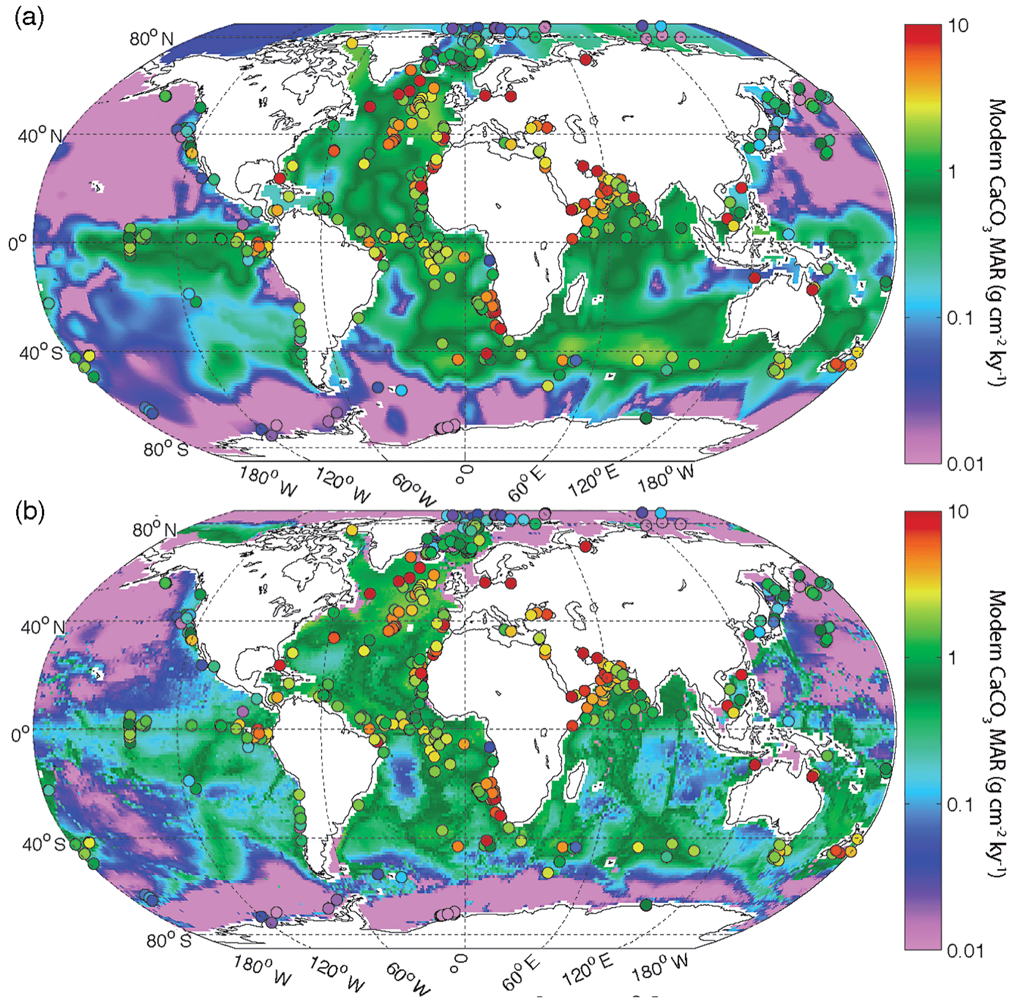
Figure 2(a) Deep-sea CaCO3 burial based on sedimentary data; (b) CaCO3 burial based on a metamodel optimized to fit the sedimentary data (Dunne et al., 2012). Filled circles show Holocene CaCO3 burial from sediment cores used in the reconstruction of past burial fluxes, using the same color scale. Note that many sediment cores were collected at sites with accumulation rates that exceed the local average sedimentation rate, a common practice to obtain high-temporal-resolution records for paleoceanographic studies (see Sects. A1 and A4 in the Appendix).
By contrast, the deep north Pacific, bathed by aged, DIC-rich waters, shows very low CaCO3 burial rates. The fraction of pelagic CaCO3 exported from the surface ocean that is eventually buried in sediments is estimated to vary between 0.6 and 0.06, depending on surface export, bottom water chemistry, sedimentary respiration rates, and lithogenic flux (Dunne et al., 2012).
Based on the modern surface sediment composition and estimates of bulk sediment burial rate, and also considering the export flux of CaCO3 from the surface ocean, the modern CaCO3 burial in deep-sea environments has been estimated to be between 100 and 150 PgC kyr−1 (Catubig et al., 1998; Sarmiento and Gruber, 2006; Dunne et al., 2012). Thus, modern estimates suggest that carbonate burial is roughly equally distributed between shallow- and deep-sea environments but with significant uncertainty in their ratio (at least a factor of 2).
2.1.3 Isotopic composition of carbonates
The globally averaged carbon isotopic signature (δ13C) of CaCO3 buried in marine sediment is surprisingly poorly constrained. While the δ13C composition of marine carbonates has been studied intensively, those studies generally consider only specific fractions of the carbonate material, such as benthic or planktic foraminifera, while the δ13C of the bulk carbonate is rarely reported. However, it is often assumed that carbonate precipitates with an isotopic composition close to that of the ambient dissolved inorganic carbon, while some modeling experiments suggests a fractionation of 0.78 ‰ as compared to ambient DIC (Kump and Arthur, 1999).
2.2 Organic carbon burial in marine sediment
2.2.1 Fluxes and fate of organic carbon in the ocean and in the sediment
The Corg buried in marine sediments is supplied by photosynthetic carbon fixation by marine phytoplankton and terrestrial plants. Marine Corg production by phytoplankton in the surface ocean has been estimated as ∼45 PgC yr−1 in pelagic ecosystems (92 % of the total ocean surface), whereas ∼9 PgC yr−1 is produced in coastal ecosystems (8 % of the total ocean surface, continental margins being defined here as regions shallower than 1000 m) (Sarmiento and Gruber, 2006 and references therein). However, only a minor fraction of the organic matter produced in the sunlit surface ocean reaches the sediment before being respired by heterotrophs (estimated as 0.34 PgC yr−1 for open ocean settings and 2.5 PgC yr−1 for continental margins; Sarmiento et al., 2002). Because organic matter is further consumed by benthic organisms on the sea floor and in the uppermost layers of the sediment, very little is permanently buried in sediments, with the highest burial fractions occurring in rapidly accumulating oxygen-depleted sediments on continental margins (Sarmiento and Gruber, 2006). Meanwhile, terrestrial organic matter may represent up to a third of the total organic matter buried in marine sediment, with the majority of terrestrial organic material burial occurring in deltaic and continental margin sediment (Burdige, 2005).
The available estimates for modern burial of Corg show large ranges. As shown by Burdige (2007), global Corg burial estimates vary by more than 1 order of magnitude (50–2600 PgC kyr−1), with several estimates significantly higher than the commonly cited range of 120–210 PgC kyr−1 (Berner, 1989; Hedges and Keil, 1995; Sarmiento and Gruber, 2006). These discrepancies are probably linked to an incomplete understanding of the sedimentary environments in coastal regions and to the different integration time of the measurements used to determine global burial on shelves (Burdige, 2007). Attempting to account for these weaknesses, Burdige (2007) suggested a total global Corg burial flux of 310 PgC kyr−1.
2.2.2 Organic carbon burial distribution in marine sediment
In contrast with CaCO3 burial, which shows relatively similar distributions between deep-sea and shelf environments, studies have generally shown that Corg burial is strongly focused over continental shelves. The reason for this contrast is that heterotrophic organisms rapidly consume organic matter, so that sinking fluxes decrease sharply with water depth, whereas carbonate minerals sink relatively unimpeded through the water column. For example, according to the estimates of Dunne et al. (2007), burial of Corg is 480 PgC kyr−1 in nearshore deposits (<50 m), 190 PgC kyr−1 on shelves (50–200 m), and 100 PgC kyr−1 on slopes (200–2000 m), greatly exceeding the burial of 12 PgC kyr−1 on deep-sea rise and plains, even though the deep-sea sediment covers nearly 90 % of the ocean floor. Burdige (2007) estimated that burial of 250 PgC kyr−1 occurs on continental margins <2000 m water depth, with a remaining 60 PgC kyr−1 in deeper waters. We note that Muller-Karger et al. (2005) estimated that roughly 40 % of the total burial occurs in margin sediments between 50 and 2000 m (ignoring the shallowest 50 m), while the remainder is buried in deep-sea sediment, which represents a much greater deep-sea burial proportion than other studies.
2.2.3 Isotopic composition of organic carbon
Because carbon stable isotope fractionation occurs during photosynthesis, organic matter δ13C is markedly different than the carbon pool from which it was formed (Degens, 1969; Freeman and Hayes, 1992). δ13C of organic matter in modern marine surface sediment reflects a variety of factors and ranges between −20 and −22.5 ‰ (Wang and Druffel, 2001). Using our database, we extracted all the δ13C measurements performed on marine sediment organic matter within the uppermost 10 cm of the sediment. We estimated the mean δ13C of organic matter in the first 10 cm of the sediment as −22.2 ‰ with a standard deviation of 2.3 ‰, consistent with prior literature (Sundquist and Visser, 2003).
2.3 Geological CO2 emissions
Modern estimates of volcanic emission of CO2 range between 6 and 14 PgC kyr−1 for mid-oceanic ridges alone (Chavrit et al., 2014) and 44 PgC kyr−1 for mid-oceanic ridges plus volcanic arcs (Coltice et al., 2004). Estimated emissions on geological timescales are notably higher, ranging from 40 to 150 PgC kyr−1 (Sundquist and Visser, 2003; Burton et al., 2013), consistent with relatively quiet volcanic activity during the late Holocene (Gerlach, 2011). It has been suggested that increased emission during deglaciations, due to mantle decompression caused by ablation of glaciers and ice caps, could have reached 200 PgC kyr−1 (Huybers and Langmuir, 2009; Roth and Joos, 2012). Continental rifting zones could also represent a significant source of exogenic carbon to the climatic system, amounting to 14 to 26 PgC kyr−1 (Lee et al., 2016). Notably, a recent study significantly increased the potential contribution of solid Earth outgassing as compared to previous estimates (see details in Burton et al., 2013 and references therein), a revision that highlights the large degree of uncertainty in this important flux.
Some reconstructions for past global volcanic activity have suggested a tight coupling between glacial ice volume and volcanic eruption frequency (Jellinek et al., 2004). Increased eruption frequency among subaerial volcanoes appears to have occurred following the highest rate of sea level rise (with a 4 kyr lag), presumably in response to mass unloading and isostatic adjustment (Huybers and Langmuir, 2009; Roth and Joos, 2012; Kutterolf et al., 2013). Subsea volcanism at mid-ocean ridges also appears to vary in response to isostatic loading as ice sheets grow and sea level drops. Lund et al. (2016) suggested that the maximum rates of seafloor CO2 emission could occur approximately 10 kyr after a sharp sea level drop, which occurred most recently at the onset of the Last Glacial Maximum (LGM) (Lambeck and Chappell, 2001; Waelbroeck et al., 2002; Grant et al., 2012), implying that peak seafloor emissions would be roughly coincident with the start of deglaciation. The isotopic composition of volcanic emissions has been estimated at around −5 ‰ (Kump and Arthur, 1999; Cartigny et al., 2001; Deines, 2002; Roth and Joos, 2012).
2.4 Erosion of continental surfaces
The second main source of geological carbon to the active pool consists in the transfer of carbon from exposed rocks through physical and chemical weathering. Carbonate rock weathering has been estimated to currently add between 70 PgC kyr−1 (Hartmann et al., 2014) and 155 PgC kyr−1 (Gaillardet et al., 1999) to the active pool, while the petrogenic particulate Corg flux to the ocean is thought to amount to between 40 PgC kyr−1 (Copard et al., 2007; Galy et al., 2015) and 70 PgC kyr−1 (Petsch, 2014). Alkalinity fluxes from the continent to the ocean also impact the carbon system. Most of the alkalinity released from the continental surface corresponds to the weathering of carbonate (63 to 74 %; Gaillardet et al., 1999), with the remainder supplied by silicate weathering. Total alkalinity fluxes to the ocean amount to between 30 Pmol equ kyr−1 (Amiotte Suchet et al., 2003) and 40 Pmol equ kyr−1 (Gaillardet et al., 1999).
The degree to which weathering varied over glacial–interglacial cycles is highly uncertain. An early modeling study estimated that global chemical erosion was 20 % higher during the LGM (Gibbs and Kump, 1994), mostly because of enhanced erosion of newly exposed continental shelves. However, Vance et al. (2009) have argued that silicate chemical weathering was much lower during glacials. It is commonly assumed that physical erosion of continental surfaces was more rapid during glacials because of enhanced action of ice sheets at high latitude (Herman et al., 2013) and the exposure of shelves, although this too has been debated (von Blanckenburg et al., 2015). It is also possible that chemical weathering could have been reduced, or changed in nature (Torres et al., 2017), due to lower temperature so that global erosion remained relatively stable over glacial–interglacial timescales (Foster and Vance, 2006).
The isotopic composition of the global erosion flux is mostly determined by the ratio of Corg to carbonate weathering and has been estimated to range between −8.5 ‰ and −5 ‰ (Kump and Arthur, 1999; Roth and Joos, 2012).
3.1 Analytical strategy overview
Sediment cores sample only a tiny fraction of the global seafloor. In order to use these unevenly distributed observations to infer integrated changes in global carbon burial, we need to take into account the following aspects: (1) the limited spatial extent that is integrated by each core; (2) the fact that accumulation rates at an individual site may not be representative of the accumulation within a broader region; and (3) the fact that carbonate accumulation rates vary widely between different parts of the world.
To account for these potential shortcomings, our quantification of global carbonate burial includes three elements:
-
The first element is an estimate of the spatial variations in global carbonate mass accumulation rate (MAR) in the modern ocean derived from sediment core tops and process modeling (Dunne et al., 2012).
-
The second element is subdivision of the ocean into coherent biogeochemical provinces, in order to account for the spatial and bathymetric heterogeneities in the sedimentary carbonate burial record. Because they take into account spatial structure in carbonate production and preservation, the province approach is likely to be an improvement over simple interpolation, especially in regions where measurements are scarce (see details in Appendix A), though future work may be useful to quantify exactly how the approaches differ.
-
The third element is reconstruction of the relative variation of the carbonate MAR in each province over time, based on a compilation of available marine sediment proxy records. These relative changes are then multiplied by the modern CaCO3 MAR estimate in each province and integrated to assess the global history of deep-sea carbonate burial (see also Cartapanis et al., 2016 for further details). We note that the last step implicitly assumes that carbonate currently present in modern sediment is in equilibrium with its surrounding environment and is not being gradually dissolved (Berelson et al., 2007) or precipitated (Sun and Turchyn, 2014), which is not universally correct. In the future, this limitation could perhaps be overcome by assimilating the observed MAR into a mechanistically based sediment module coupled with carbonate production and ocean chemistry, though this is beyond the scope of the present work.
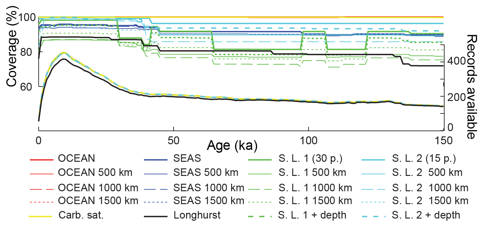
Figure 3Coverage and number of records used for each province map. Coverage is calculated by summing the modern burial rates in each province (Fig. A1) for which at least one sedimentary record is available, divided by the modern burial flux. The modern map used corresponds to Fig. 2a.
3.2 Modern carbonate MAR map
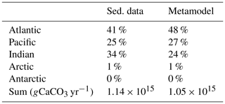
We use two different but closely related maps of modern carbonate MAR (Fig. 2), both of which were previously published by Dunne et al. (2012). The first is based only on observations and was determined by multiplying the carbonate concentration in surface sediments by the bulk sediment accumulation rate. The carbonate concentration map was generated by combining several literature sources (Seiter et al., 2004; Dunne et al., 2007), whereas the bulk MAR map was determined based on the geometric mean of two pre-existing maps (Jahnke, 1996) and other unpublished data; see details in Dunne et al. (2007, 2012). It is important to note that the observationally based estimates of both the carbonate concentration and MAR have insufficient spatial resolution to adequately resolve continental margins (Fig. 2a). The second map was generated using a metamodel derived from a process-based approach (including satellite-derived carbonate export production and water-chemistry-dependent dissolution in the water column and sediments) that was minimally tuned using the sedimentary data (Dunne et al., 2012). The metamodel map shows similar patterns in the deep sea but better resolves the bathymetric imprint on carbonate preservation (Fig. 2b). The two approaches provide slightly different spatial distributions of burial, allowing a test of the sensitivity of our reconstructions to this uncertainty (see Table 1). Although the absolute values differ, the relative changes in our reconstructed global carbonate burial over time are insensitive to the choice of maps (see Appendix A).
Table 1Estimates of the modern global deep-sea CaCO3 burial flux. The fractional contribution of each basin is shown, in percent, and the total estimated burial flux shown in g CaCO3 yr−1. The two columns correspond to the two estimates shown in Fig. 2, and the basin areas correspond to province map 1 shown in Fig. A1.
The two modern maps attempt to accurately represent the spatial distribution of the modern CaCO3 burial flux. Sediment cores, however, are often situated to target rapidly accumulating depocenters in order to provide greater temporal resolution for paleoceanographic reconstructions. As a result, we expect a bias towards high accumulation rates, which is confirmed in Fig. 2. We address this sampling bias when evaluating uncertainties (see Sects. A1 to A4).
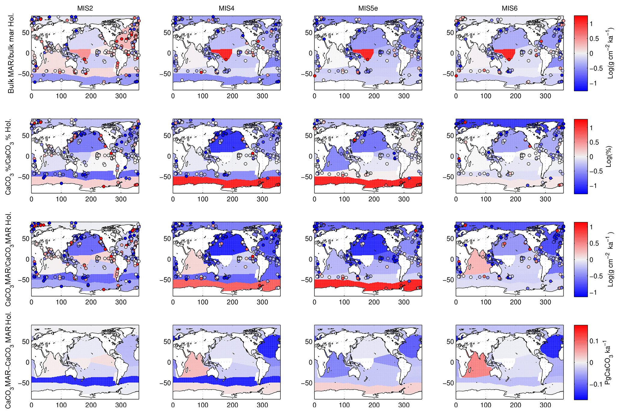
Figure 4Example of calculated changes in deep-sea sedimentation relative to the Holocene using one province map. The first three rows show relative changes in bulk sediment MAR, carbonate content, and carbonate MAR, while the last row shows absolute changes in carbonate MAR. Changes are shown for the LGM and Marine Isotope Stages 4, 5e, and 6. Note that the absolute carbonate flux refers to the integrated burial over the province (not area normalized). The modern map used here corresponds to Fig. 2a, and the province map is S.L.2. Note that the data shown here are not corrected for the long-term trend of accumulation rate, as the correction is calculated and applied at the global burial level.
3.3 Relative changes in burial rate from sediment core database
We created a database including surface- and downcore sediment datasets, retrieved from the National Oceanic and Atmospheric Administration (NOAA) (ftp://ftp.ncdc.noaa.gov/pub/data/paleo/paleocean/sediment_files/, last access: Mai 2015) and PANGAEA (http://www.pangaea.de, last access: Mai 2015) online repositories. All the datasets that contained CaCO3 concentrations, CaCO3 accumulation rates, age models and sediment density values were taken into consideration (for a complete detailed description of the procedure and quality control, the reader is referred to Cartapanis et al., 2016). Whenever available, 230Th-normalized sediment accumulation rates were used. Where these measurements were not available, sedimentation rates were determined at the depth of each carbonate measurement from the reported age–depth relationship. When possible, we used reported dry bulk density values. Otherwise, we assumed a constant value of 0.9 g cm−3 to convert linear accumulation rates to MAR. Each sedimentary record was expressed as a fraction of the respective mean Holocene value.
The mean LGM : Holocene (18–25 and 0–10 ka, respectively) ratio was determined for each province and multiplied by the corresponding modern burial rate to estimate the absolute value of carbonate burial during the LGM. Note that we used the geometric mean of available records in each province, given that the LGM : Holocene ratios of individual cores are log-normally distributed. Moreover, if in a single province we have two MAR records, one showing 2 times higher MAR during the glacial, while the other showed only half of modern during the glacial, the best guess would be that the true change in sedimentation was negligible. This is better represented by the geometric mean of (2, 0.5) = 1 (no change), whereas the arithmetic mean (2, 0.5) = 1.25 would bias the result toward high values. The carbonate burial of all provinces is summed to provide the LGM global burial rate.
The same procedure was applied to calculate global carbonate sediment content and bulk MAR at every 1 kyr time step over the past 150 kyr. Any time interval within a sediment record for which no measurement was present over a period longer than 10 kyr was excluded from the calculation of the regional stacks, leading to a total of 637 sediment time series, from which 370 records were used to calculate the LGM : Holocene ratio (Figs. 3–4), while 170 to 130 records were used for periods older than 40 kyr. When no record was available for a specific province and/or for a specific time period, the province flux was assumed to be constant and equal to modern values. The provinces for which no downcore record was available represent 0 % to 18 % of the ocean surface, corresponding to 0 % to 12 % of modern burial (this metric will be referred as “coverage” in the following discussion) for the LGM (18–25 kyr; Fig. 3). As a consequence, the reduction of the coverage during older periods tends to diminish the difference from the modern situation, a conservative assumption that may bias our reconstruction toward smaller changes than actually occurred. The available records are distributed over the entire depth range (100 records shallower than 1000 m, 103 records between 1000 and 2000 m, 137 records between 2000 and 3000 m, 290 records between 3000 and 4000 m, and 106 records below 4000 m deep).

Figure 5CaCO3 MAR time series, considering different aspects of variability. (a) Bulk sediment MAR time series distribution based on the 20 province-map scenarios (mean, black line; ±1σ, red area; ±2σ, blue area), and the distribution of the long-term trend correction for each province map (mean, black line; ±1σ, dark grey; ±2σ, light grey) using a least-squares spline model. (b) Bulk sediment MAR as in panel (a) but with the modeled long-term trend removed. (c) Global CaCO3 MAR reconstruction without detrending. (d) Global CaCO3 MAR reconstruction calculated only from variations in CaCO3 concentration, assuming a constant bulk sedimentation rate. (e) Global CaCO3 MAR reconstruction obtained from the bulk MAR and variations in CaCO3 concentrations. Panel (f) is the same as (e) but with MAR corrected for the long-term trend. In all panels, the thin black lines correspond to the 20 individual province-map scenarios. The modern map used for all calculations corresponds to Fig. 2a.
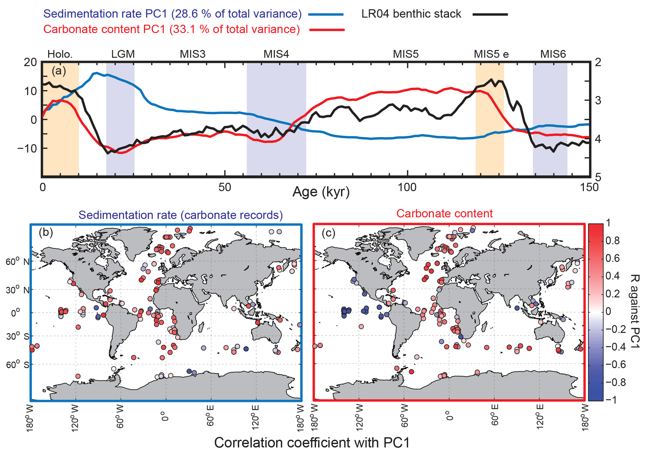
Figure 6Principal components of temporal variation in sediment mass accumulation rates and CaCO3 concentrations. The first principal component (PC1) is displayed in panel (a) for both sedimentation rates and carbonate content, and explains 28.6 % and 33.1 % of the total variance, respectively. Yellow vertical bars correspond to Holocene and MIS5e; blue vertical bars are for LGM, MIS4, and MIS6. Panels (b) and (c)show the correlation coefficients for individual records of sedimentation rates and carbonate content, against their respective PC1. In this analysis, we used only records that cover 80 % of the studied interval.
3.4 Assessing changes in deep ocean MARs and their role on the global estimates
Since carbonate MAR depends on both the sedimentation rate and sedimentary carbonate concentration, we first calculate the global bulk MAR by considering only relative changes in the sedimentation rates and a modern bulk MAR map (Jahnke, 1996). This reconstruction (Figs. 4, 5A, and Table 3) shows generally higher bulk sediment burial during peak glacials and deglaciations, broadly consistent with previous studies (Covault and Graham, 2010). However, the reconstructions display a pronounced increasing trend towards the present for all the province-map scenarios (Fig. 5A). This is partly due to the absence of density data for many cores, which tend to underestimate burial for older, more compacted sediment. Moreover, the apparent sedimentation rate decreases as a power–law function of the intervals between two age controls (Schumer and Jerolmack, 2009), suggesting that sedimentation rates are likely underestimated as age increases, when the age model accuracy is generally lower compared to more recent periods.
Because of the lack of density information for individual cores, we chose to correct for compaction at the global scale by assuming that the global bulk burial rate was equal during the late Holocene and Marine Isotope Stage 5e (MIS5e), and subtracting the intervening trend, an assumption that could be revisited in future work as more information becomes available. Given this assumption, we corrected the long-term trend of the global aggregate bulk sedimentation rate for each province map using a least-squares spline (Fig. 5a and b). The detrended CaCO3 MAR reconstruction (Fig. 5f) is much more similar to the globally flux-weighted CaCO3 concentration record (Fig. 5d) and suggests that global bulk MAR in deep-sea sediment peaked during glacial maxima and deglaciations, as well as during MIS4: 114 %, 104 %, and 105 % relative to the Holocene MAR for the LGM, MIS4, and MIS5e (119–124 ka), respectively. The LGM-to-Holocene change is consistent with, but smaller than, a recent estimate (125 % ± 15 %) using a smaller but partially overlapping set of cores that included Corg measurements (Cartapanis et al., 2016).
We performed a principal component analysis (PCA) on the MAR time series in order to assess the overall spatial and temporal variability (Fig. 6). For this calculation, we used only the records that cover at least 80 % of the studied interval. The first principal component (PC) of the bulk MAR shows variability that is similar to the bulk MAR reconstruction, and the sedimentation rate time series are broadly correlated with the sedimentation rate PC1, without showing any consistent geographic pattern.
We then performed a similar analysis, using only the relative changes in the sedimentary carbonate concentration (assuming constant sedimentation rates), and the modern carbonate MAR map as a reference (Dunne et al., 2012). This analysis shows that the CaCO3 content in deep-sea sediment (weighted by modern carbonate MAR) was consistently lower during glacials compared to interglacials, with the lowest values reported during MIS4 and MIS2 (Figs. 4, 5d, and 6). The first PC of the carbonate content records is similar to the global reconstruction, and the correlation map between CaCO3 concentration time series and CaCO3 concentration PC1 shows a clear antiphasing between the eastern Pacific and the rest of the world ocean (Fig. 6). While CaCO3 concentrations were lower during the glacial in the Atlantic, they were substantially higher in the eastern Pacific.
In order to assess the impacts of variations of both bulk MAR and CaCO3 concentration in our reconstruction, we calculated global carbonate MAR variations using two different methods. First, we calculated global CaCO3 MARs using the relative changes in individual sedimentary carbonate MAR time series (Figs. 4, 5c). Second, we made the simpler calculation of taking the product of the reconstructed CaCO3 concentration with the average relative changes in bulk MAR reconstruction for each scenario (Fig. 5e).
As both methods provided very similar results, we calculated CaCO3 MAR using the simpler of the two, taking the product of the relative changes in corrected bulk sediment MAR (Fig. 5b) and the reconstruction of CaCO3 concentration (Fig. 5d). This final reconstruction (Fig. 5f; see details in Fig. A4) thus accounts for variations in the bulk MAR, as well as variations in the concentration, and is corrected for the long-term trend directly inferred from the bulk MAR.
As shown in Fig. 5f, the reconstruction indicates that global mean deep-sea CaCO3 burial was not significantly different from the present day during MIS5, dropped to the lowest rates during MIS4, and then remained below interglacial rates until the deglaciation. In part, the similarity of CaCO3 burial between MIS5 and the Holocene reflects our assumption that bulk sediment MARs during MIS5 and the Holocene were similar, which underlies our detrending. However, MIS5 and the Holocene are also indistinguishable in the burial flux reconstruction estimated from CaCO3 concentration alone (Fig. 5d), in which MIS4–MIS2 also stand out as having significantly reduced burial.
4.1 Mass-balance calculation
In order to estimate the impact of the reconstructed carbonate flux on the carbon and alkalinity budgets, we made a simple running-sum calculation of carbon and alkalinity sources and sinks over the full last glacial cycle. We did so within the numerical framework of a simple three-box model (three oceanic boxes and the atmosphere) using the input and output fluxes for both carbon and alkalinity as illustrated in Fig. 1 and model settings described in Toggweiler (1999) following the equations detailed in Sarmiento and Toggweiler (1984). Briefly, the model tracks the mass budget for inorganic carbon in three well-mixed ocean boxes (surface high and low latitudes, and deep ocean) and in the atmosphere. The C cycle is linked to the cycles of alkalinity and nutrients (phosphate) in the ocean boxes. For simplicity, nutrients are prescribed in the surface boxes, and water mass transport between boxes is kept constant. Exchange of CO2 between the surface boxes and the atmosphere exchange is based on aqueous carbon chemistry and a constant piston velocity (Sarmiento and Gruber, 2006). The deep-sea [] concentration was calculated based on aqueous carbon chemistry (Sarmiento and Toggweiler, 1984; Dickson and Goyet, 1994) and can be very well approximated by the difference between dissolved inorganic carbon and alkalinity. We emphasize that the use of the three-box model here only provides a very small modification of the results obtained with the simple running sums, providing average deep ocean values that vary slightly due to changes in air–sea partitioning; very similar results would be obtained by considering simply the mass balance of global alkalinity and carbon inventories, without calculating their distributions between ocean and atmosphere.
The two input fluxes to the active pool are the geological outgassing of CO2 and the erosion of continental surfaces (due to the dissolution of carbonate and oxidation of sedimentary Corg), while the four output terms represent carbon burial in sediment divided into four components: both Corg and CaCO3 for each of the shelf and deep-sea environments. The input flux of alkalinity is assumed to be due to the erosion of continental surfaces, including both carbonate and silicate weathering, while the flux out of the system is given by burial of CaCO3 in marine sediment.
Our mass-balance simulations prescribe a range of possible scenarios for variable input and output fluxes, in order to estimate the resulting transient changes of carbon and alkalinity inventories and δ13C. The deep-sea burial fluxes are derived from our sedimentary reconstructions, while the shelf burial fluxes and the input flux are varied in order to illustrate hypothetical (yet realistic) scenarios. In total, we include eight different scenarios to illustrate the impact of each variable in isolation, as well as in combination with others (Table 3). In all cases, we vary the fluxes over feasible ranges using a Monte Carlo approach (1000 transient simulations per experiment).
It is important to note that we do not consider temporally variable erosion fluxes but instead hold them constant over time in any given simulation, due to a paucity of consistent observational constraints. The work of von Blanckenburg et al. (2015) argued that erosion was, indeed, constant over glacial cycles, while others have argued that erosion was lower (Vance et al., 2009) or higher (Herman et al., 2013) during glacials. Erosion contributes both carbon and alkalinity, and although it remains difficult to evaluate the global impacts of changes in erosion, they may have been substantial.
A key feature of the simulations is that they assume long-term balance over a full glacial cycle. The fact that CO2 and δ13C display very stationary mean values over several glacial cycles (Zeebe and Caldeira, 2008) suggests that the system is indeed close to steady state over each full glacial cycle, so that the assumption is unlikely to introduce a large bias. Therefore, assuming that the system was at steady state over the last glacial cycle, we calculated the input fluxes of carbon and alkalinity that would have been necessary to balance the prescribed burial (as well as prescribed input changes, if any) over the full glacial cycle for a given scenario and provided those as a constant input flux throughout the cycle. Thus, although the carbon and alkalinity fluxes are out of balance at each point within the cycle, they always integrate to zero net change between 0 and 123 kyr. Similarly, the isotopic composition of the system is prescribed by setting the δ13C of the erosion flux at a value that balances the other fluxes, consistent with the long-term steady-state assumption. Although forcing the carbon isotopes to be equal at start and end points does ignore a small long-term drift in whole-ocean δ13C (Oliver et al., 2010), it provides a clearer illustration of the isotopic implications of inventory changes over a single glacial cycle. We note that this strategy results in different total input fluxes (and therefore different residence times of the active pool) for each experiment.
To account for uncertainties in the modern fluxes (Fig. 1), the relative changes in the prescribed time series are multiplied by an estimate of the global modern flux, which is generated using a distribution that represents the uncertainty in modern global burial estimates (see Table 3, and Appendix B and Fig. A6). The forcing thus accounts for our reconstruction and their uncertainties, as well as the uncertainties in the modern burial estimates. The same procedure was applied for Corg burial variations in the deep ocean as shown in Cartapanis et al. (2016) but using a different distribution (Table 3; see details in Fig. A6).
In the following sections, we consider eight different scenarios in which we calculate the total mass and δ13C of the active carbon pool, as well as the oceanic alkalinity inventory, according to different combinations of temporally varying input and output fluxes for carbon and alkalinity. In experiments 1 and 2, we isolate the impact of reconstructed deep ocean inorganic (this study) and organic carbon burial (Cartapanis et al., 2016), respectively, and combine them in experiment 3. Experiment 4 only considers scenarios for shelf burial variations, while experiment 5 combines experiments 3 and 4, thus including variations of burial in both deep and shallow environments. Experiment 6 depicts a hypothetical deglacial carbon pulse based on Huybers and Langmuir (2009) and is combined with experiment 3 (burial in the deep sediment) in experiment 7, and with experiment 5 (burial in deep and shallow sediments) in experiment 8. Thus, these scenarios incrementally explore the impact of the different forcing and their interactions on the carbon and alkalinity budgets over the last glacial cycle.
Table 2Summary of estimated changes in carbonate MAR for each province map. The number of records used, mean coverage (%), and mean MAR (in % of modern value) are shown for four intervals (LGM, MIS4, MIS5e, and MIS6) for each province map. The results correspond to the calculations of temporal variability shown in Fig. 5f. The modern burial map used for all calculations corresponds to Fig. 2a.
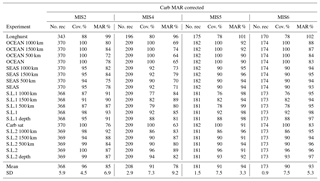
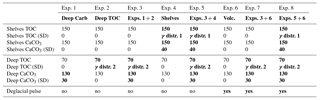
Table 3Modern burial distribution (PgC kyr−1) used for the Monte Carlo simulations (mean and standard deviation). When the distribution type is not specified, a normal distribution was used. Boldface indicates variable fluxes over time. Results of experiments 1 and 2, 3 to 5, and 6 to 8, are shown in Figs. 7, 8, and 10, respectively. The gamma distributions (γ distribution) used for Corg burial are shown in Fig. A6.
4.2 Deep-sea burial impact on carbon and alkalinity inventories (experiments 1 to 3)
Assuming a constant alkalinity flux to the ocean, and all other factors being equal, our reconstruction of deep-sea CaCO3 burial in the deep ocean coupled with uncertainties in modern fluxes (Table 2) implies changes in the alkalinity inventory that could reach up to 100 µequ kg−1, with a minimum centered around ∼70 kyr near the MIS4/MIS5 transition, gradually rising to a maximum during the early deglaciation at ∼15 kyr (Fig. 7a, experiment 1). This increasing trend is a robust consequence of the low reconstructed carbonate burial from MIS4 to MIS2, with a most probable amplitude of 70±30 µequ kg−1. Note that the [] changes shown in all of our experiments ignore possible changes in ocean circulation or biology, and they do not consider contributions to alkalinity other than and , and are therefore not expected to be accurate – they are simply illustrations of the purely inventory-driven expectations of deep-sea [] change. The actual realized changes of [] that occurred over the last glacial cycle have been shown to have been quite small (Yu et al., 2010), which would reflect the net result of any inventory changes plus other processes such as ocean circulation and biology-driven changes.
Changes in Corg burial in the deep sea followed a markedly different progression, with larger (rather than smaller) burial during peak glacial and deglaciation (Cartapanis et al., 2016), causing the C inventory to rise over MIS5 by 400 (150 to 950) PgC, equivalent to 20 (10 to 50) µmol kg−1 in the global ocean (Fig. 7b, experiment 2), and to decrease by the same amount from MIS3 to the early Holocene. Summing the two deep-sea burial fluxes together leads to a slightly muted change in the carbon inventory (Fig. 8a, experiment 3). The changes in deep-sea Corg burial would have decreased the isotopic composition of the active carbon pool during the early glacial, by 0.2 (0.1 to 0.5) ‰ during MIS4, but with a negligible change between LGM and the late Holocene (Fig. 8a). It is important to note that, for these three first experiments, the mean C input flux required to compensate for the outputs is close to 500 PgC kyr−1, which exceeds the standard estimates for present-day carbon input (160–400 PgC kyr−1; Fig. 1). This discrepancy arises from the relatively large estimates of present-day carbon burial, combined with the absence of much lower deep-sea burial fluxes during the glacial – either the present-day input fluxes are underestimated, the present-day burial is overestimated, or there were additional changes in the fluxes over the glacial cycle. Thus, we turn next to possible changes in burial on the shelves.
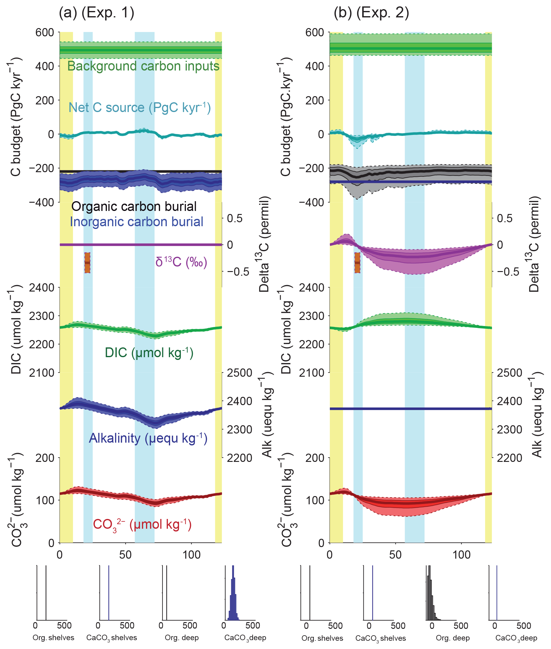
Figure 7Simulated impacts of reconstructed deep burial fluxes on carbon and alkalinity inventories: (a) variable deep-sea CaCO3 burial and (b) variable deep-sea Corg burial. For each panel, the uppermost curves show the carbon budget terms (constant background carbon input, organic, inorganic carbon burial, and net flux from the geological to the active carbon reservoir) used to force the simulations. For each time series, the mean of the scenarios (thick line), ±1σ, and ±2σ are shown. Below are shown the simulated δ13C of the total active carbon pool, deep ocean alkalinity, deep ocean DIC, and implied deep ocean [] (µmol kg−1). The [] only reflects changes in the alkalinity and DIC inventories, not changes in ocean circulation or biology. An estimate for the whole-ocean δ13C by Peterson et al. (2014) during the LGM is also shown in orange (with upper and lower estimates). Vertical bars highlight cold periods (MIS2/LGM and MIS4) in blue and full interglacial conditions (Holocene and MIS5e) in yellow. The distribution of the modern fluxes used to drive the scenarios is shown by the histograms at the bottom of each panel.
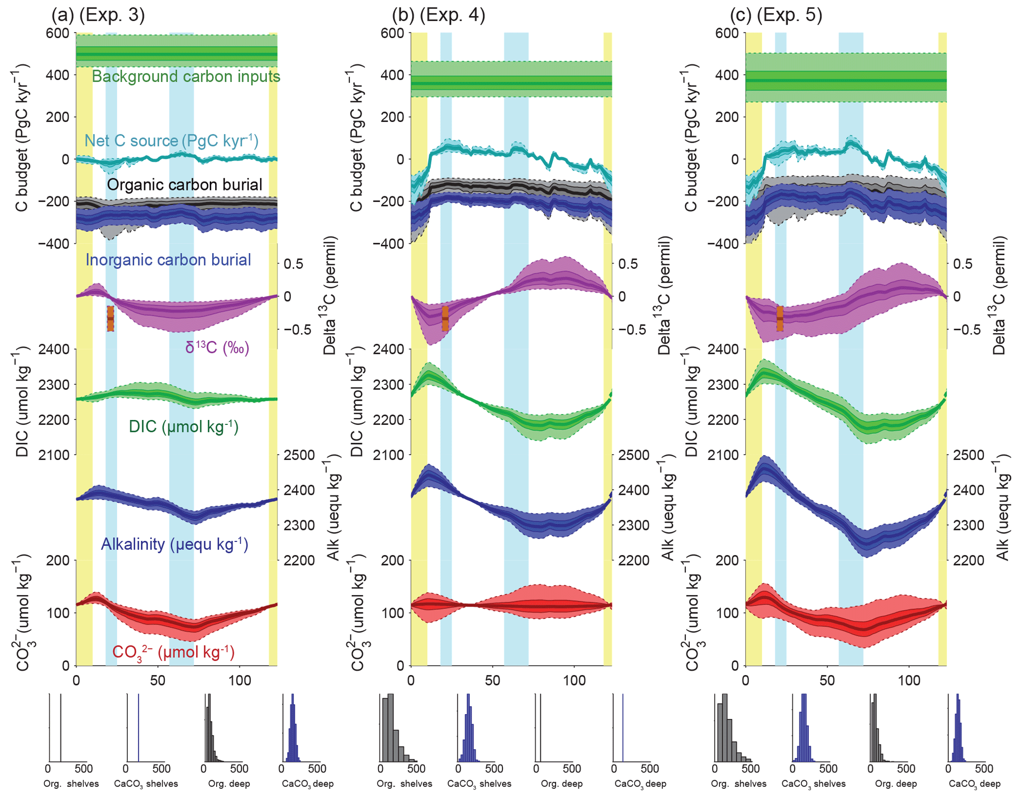
Figure 8Simulated impacts of deep and shelf burial fluxes on carbon and alkalinity inventories: (a) variable deep-sea burial (carbonate plus Corg), (b) variable shelf burial, and (c) variable total marine burial (deep plus shelf). All quantities and bars are plotted as in Fig. 7.
4.3 Shelf burial impact on carbon and alkalinity inventories (experiments 4 and 5)
The burial of CaCO3 and Corg on continental shelves depends both on their production rate and their preservation. Preservation is particularly difficult to estimate, given the importance of sediment transport and redeposition in dynamic coastal environments. Here, we use the very simple illustrative assumption that, globally, the burial over shelves was linearly proportional to the changes in the surface area available for sediment production and accumulation. Although this is a gross simplification of reality, and may overestimate the actual changes, it allows a first-order estimate of the potential magnitude of shelf burial changes on the global carbon cycle (Wallmann et al., 2016).
We calculated the relative changes in the surface area bounded by the 0 and 100 m isobaths as well as the 0 and 200 m isobaths over time, using ETOPO01 (Amante and Eakins, 2009) and a global sea level reconstruction curve (Grant et al., 2012). Because of the distribution of the global hypsometric curve (Fig. 9a), the surface area of the 0–100 m depth range was reduced by up to 60 % during the last glacial, which is certain to have led to reduced burial (Fig. 9b), consistent with Vecsei and Berger (2004).
Our results show that variations of Corg and CaCO3 burial fluxes driven by changes in sea level could have increased DIC and alkalinity inventories by up to 150 µmol kg−1 and 150 µequ kg−1 from MIS5 to the last deglaciation, because of reduced burial during times of lower sea level (Fig. 8b, experiment 4). The ALK and DIC inventories change in parallel because of our assumption that both burial fluxes would have varied in proportion to the shelf area, which leads to relatively small changes in the [] (the difference between DIC and ALK). Despite these parallel changes, the fact that Corg burial is strongly focused in shallow environments, in contrast to the equal partitioning of carbonate burial between shallow and deep environments, means that the global proportion of Corg to carbonate burial would have varied with changing shelf area (Wallmann et al., 2016). Our calculations suggest that the relative reduction of Corg burial cause by limited shelf area during glacials would have lowered the δ13C of the active carbon pool by up to 1 ‰ from MIS5 to the early deglaciation. The large uncertainties in modern burial fluxes result in large uncertainties in the ratio of DIC : ALK changes, with important implications.
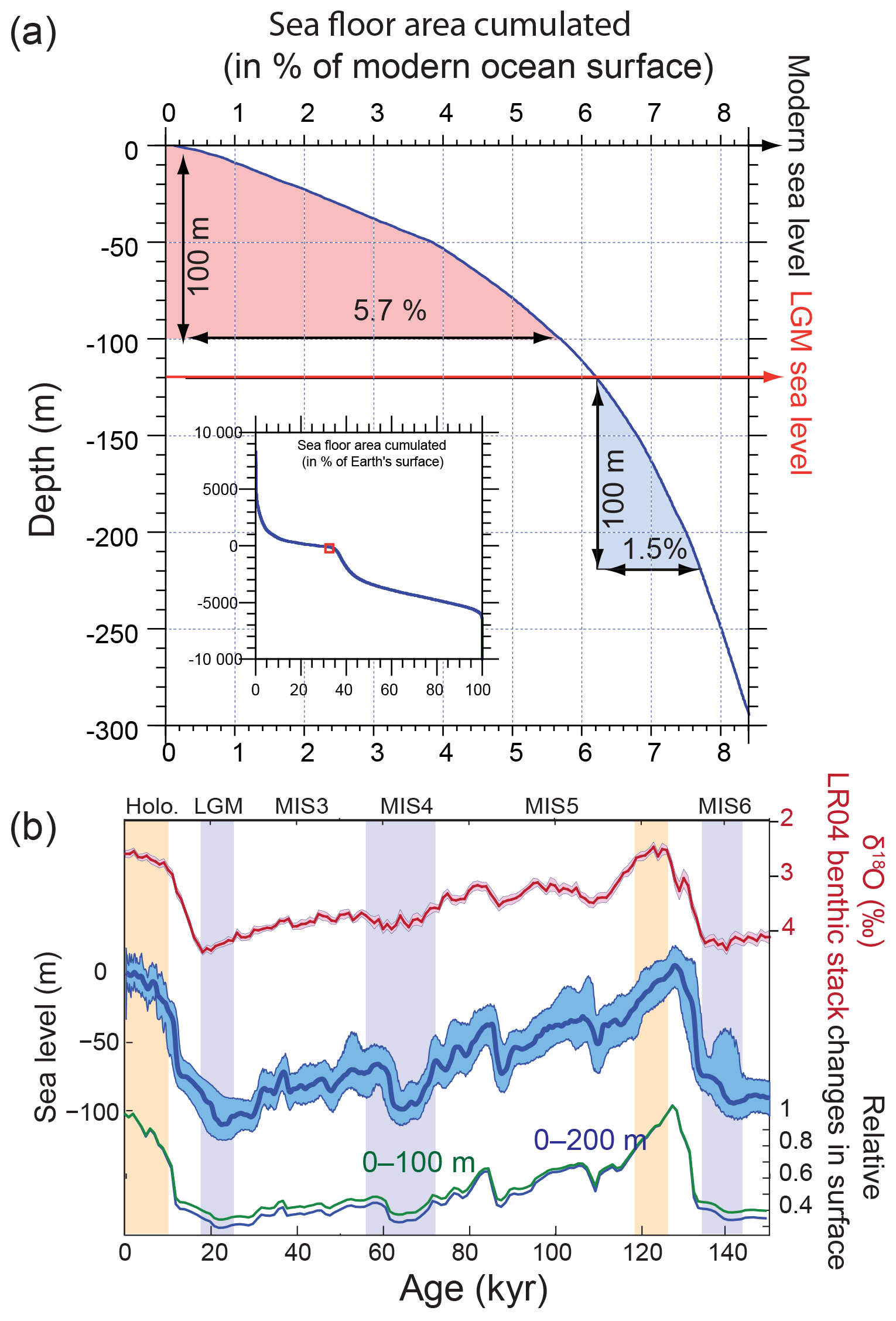
Figure 9(a) Global hypsometric curve based on ETOPO01 (Amante and Eakins, 2009); (b) LR04 benthic stack (Lisiecki and Raymo, 2005); sea level reconstruction (Grant et al., 2012); and calculated changes in the surface of the 0–100 and 0–200 m depth intervals relative to the modern situation. Vertical bars are as in Fig. 6.
4.4 Combined impact of sedimentary burial and carbon input variations (experiments 6 to 8)
It has been suggested that the rate of carbon input to the active pool from volcanic sources increased during glacial maxima (Lund et al., 2016; Ronge et al., 2016) and/or deglaciations (Huybers and Langmuir, 2009; Stott et al., 2009). Note that, for the purpose of this discussion, we consider peatlands and permafrost part of the “active” pool but not surficial marine sediments. The magnitude of these postulated volcanic carbon input variations is highly uncertain, and reconstructions of relative changes in subaerial volcanic outgassing rates over time suggest that the volcanic carbon input was notably delayed, relative to the deglacial increase in PCO2 recorded in ice cores, requiring other mechanisms to be important at this time (Huybers and Langmuir, 2009; Roth and Joos, 2012). Nonetheless, it would appear likely that changes in geological carbon inputs over the glacial cycle were significant. We do not attempt to provide an exhaustive test of the existing hypotheses for temporally variable carbon input. Instead, we simply apply a pulse of carbon input to our mass-balance calculation during the deglaciation, which follows the temporal changes given by the reconstruction of changes in terrestrial volcanic emission (Huybers and Langmuir, 2009) to produce an illustrative variable carbon input to the active pool.
As shown in Fig. 10a (experiment 6), the simulation with only variable carbon input produces similar results over the deglaciation to those estimated by Huybers and Langmuir (2009) (see also Roth and Joos, 2012). However, within our broader perspective, it is clear that, when viewed over the glacial cycle (and given our requirement that the carbon inventory be the same at the beginning and end of the cycle), a major effect of a temporally variable carbon input is to lower the implied background input rate. As a result, the carbon inventory gradually declines from interglacial to glacial maximum, and is then rapidly increased by the volcanic pulse (Fig. 10a).
When our reconstructed deep burial variations are also included, the magnitude of the MIS5–MIS4 [] peak is reduced relative to the deep-burial-only case (Fig. 10b, experiment 7). When shelf burial changes are also included, the mean carbonate ion variations are altered little, but the δ13C changes significantly (Fig. 10c, experiment 8). In this case, the δ13C of the ocean during the LGM is similar to that observed, even with no change in the terrestrial biosphere, as discussed further below.
Notably, only the experiments including variable shelf burial (Figs. 8b, c, and 10c) simulate Holocene input fluxes that overlap with the observational estimates summarized in Fig. 1. This is because only the variable shelf experiments provide a sufficient reduction of carbon burial fluxes during glacial periods to allow the full cycle carbon budget to be balanced with the relatively small modern estimates of the carbon input fluxes. Although this should not be taken as proof that the changes are correct, it shows encouraging consistency with the reconstructed and conjectured evolution of the carbon inventory over time.
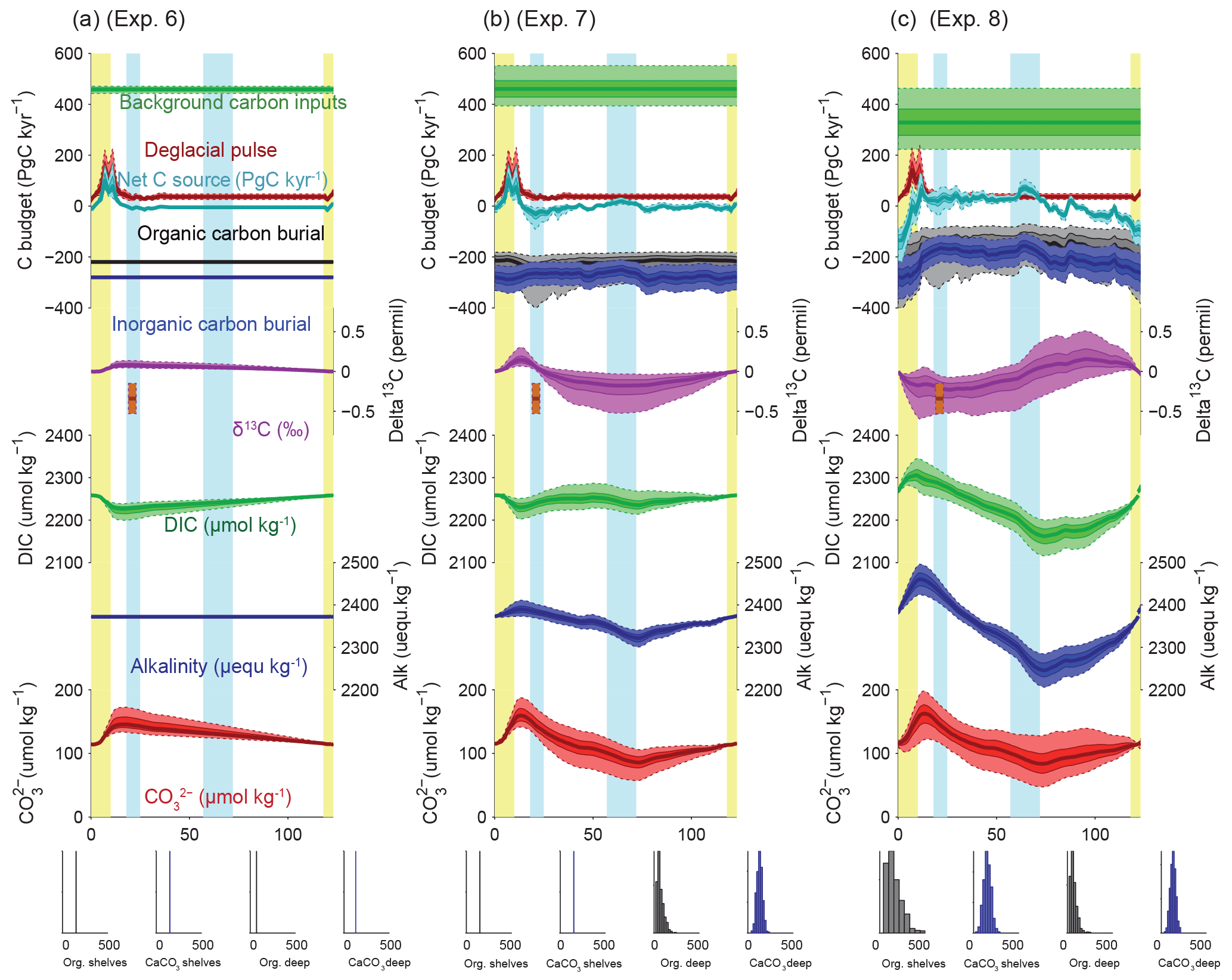
Figure 10Simulated impacts of variable burial and outgassing fluxes on carbon and alkalinity inventories: (a) deglacial carbon input pulses, (b) variable deep-sea burial plus deglacial carbon input pulses, and (c) all variable (deep-sea burial, shelf burial, and deglacial carbon input pulses). All quantities and bars are plotted as in Fig. 7, with the addition of time-varying carbon input pulses based on subaerial volcanic emission (Huybers and Langmuir, 2009) in red.
5.1 Carbonate burial in the deep ocean
The calculations shown above are based on individual time series of CaCO3 MAR from hundreds of sediment cores, using previously reported sedimentary CaCO3 content, sedimentation rates, and dry bulk density when available (see Supplement). Following the method of Cartapanis et al. (2016), we used these individual records to calculate, at each 1 kyr time step over the past 150 kyr, the CaCO3 MAR in oceanographically defined provinces as a fraction of their Holocene values. Notably, these sediment cores record the actual realized burial, not just a proxy thereof. Although the preserved record may underrepresent transient deposition and dissolution events, and the available sediment cores are undoubtedly subject to multiple biases (Appendix A), our broad spatial reconstruction should tend to minimize locally obfuscating factors, providing a more robust reconstruction of carbonate burial, globally. Absolute changes in CaCO3 burial were obtained by scaling reconstructed relative changes in CaCO3 MAR to the modern MAR (Figs. 2 and A1). Uncertainty in the global burial flux was estimated using a bootstrap technique (Appendix A). The resulting reconstruction is sure to contain biases and will hopefully be improved in future; however, it represents the most comprehensive such undertaking to date and it is not obvious to us how the reconstruction could be improved significantly without a major expansion of the existing dataset.
As shown in Fig. 11, the reconstruction indicates that global mean deep-sea CaCO3 burial was not significantly different from the present day to MIS5, dropped to the lowest rates during MIS4, and then remained below interglacial rates until the deglaciation. The spatial pattern of change, which displays the well-known deep Pacific–Atlantic antiphasing (Farrell and Prell, 1989; Hain et al., 2010) (Fig. 6), is consistent with a previously reported shoaling of well-ventilated North Atlantic Deep Water (NADW) (Boyle and Keigwin, 1982; Curry et al., 1988; Labeyrie et al., 1992; Lynch-Stieglitz et al., 2007; Guihou et al., 2011) and an enhanced soft tissue pump at the start of MIS4 (Kohfeld and Chase, 2017). The associated increase of DIC-rich Antarctic Bottom Water (AABW) would have decreased [] and favored the dissolution of CaCO3 in deep Atlantic sediments. An increased rain of organic matter to the deep sea, or a change in the rain ratio, such as what may have resulted from a postulated shift toward proportionally more siliceous phytoplankton (Brzezinski et al., 2002) or a midlatitude temperature decrease (Dunne et al., 2012), could have accentuated the DIC increase (Boyle, 1988; Hain et al., 2010; Yu et al., 2014; Galbraith and Jaccard, 2015).
Consequently, the reduced rate of alkalinity removal in the Atlantic during the glacial would have increased the total alkalinity inventory of the ocean, which would be expected to have increased [] and consequently carbonate preservation elsewhere, a compensation long understood to have occurred in the Pacific Ocean (Farrell and Prell, 1989) and consistent with our observed Atlantic–Pacific antiphasing. However, our calculations suggest that reduced burial in the Atlantic Ocean during the last glacial was not entirely compensated in the Pacific Ocean, leaving glacial carbonate burial rates lower than for the Holocene (Figs. 6 and 11). This implies that, if the alkalinity inputs from weathering had remained constant (as assumed in our mass-balance calculations), excess alkalinity in the global ocean would have built up during glacials as compared to interglacials. Additionally, despite notable pulses of CaCO3 burial in the deep ocean in some locations during the deglaciation (Jaccard et al., 2005; Dubois et al., 2010; Rickaby et al., 2010; Jaccard et al., 2013), and in contrast with expectations (Broecker and Peng, 1987; Boyle, 1988; Sigman and Haug, 2003), our reconstructions suggest that preserved deep-sea CaCO3 burial itself did not drastically peak during the last deglaciation, although post-depositional dissolution cannot be excluded.
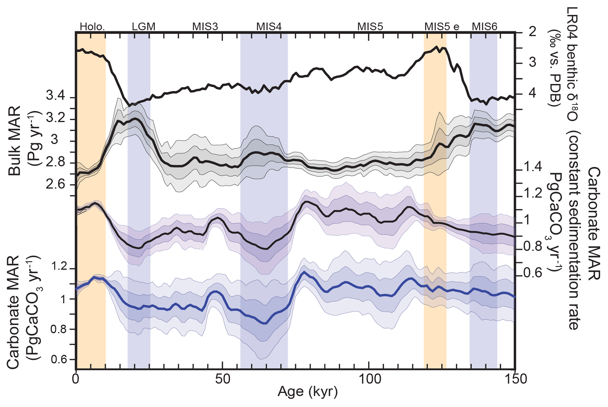
Figure 11Global changes in deep-sea carbonate burial over the last glacial cycle. Curves show, from top to bottom, a global stack of benthic foraminifera δ18O (Lisiecki and Raymo, 2005); reconstructed bulk sediment MAR; CaCO3 MAR assuming constant sedimentation rate; CaCO3 MAR using reconstructed sedimentation rate. The latter three curves show the mean, ±1σ, and ±2σ; see details in the Supplement). Vertical bars highlight cold periods (MIS2/LGM, MIS4, and MIS6) in blue and full interglacial conditions (Holocene and MIS5e) in yellow.
5.2 Changes in deep-sea []
The fact that deep-sea CaCO3 burial did not increase during the glacial, despite the loss of marginal carbonate depocenters on shelves due to sea level fall, may seem counterintuitive. If the alkalinity input flux from weathering had remained constant (Gibbs and Kump, 1994), the loss of the coastal alkalinity sink should have led to a buildup of ocean alkalinity and a compensatory increase in deep-sea CaCO3 burial (Opdyke and Walker, 1992). However, this chain of expectations does not consider possible increases in the DIC of the deep sea that could have counterbalanced the impact of an alkalinity increase on the [] there. Because the [] is dependent not only on ALK but also on DIC (since [] ≈ ALK – DIC), large changes in DIC will cause [] to change in addition to changes caused by variations in ALK. In fact, it seems likely that deep-sea DIC changes would have arisen both from enhanced carbon sequestration by saturation, soft tissue and disequilibrium carbon storage (Eggleston and Galbraith, 2018; Ödalen et al., 2018), and changes in the active carbon inventory (Yu et al., 2013).
As mentioned above, our mass-balance calculations resolve only changes in the total inventories due to geological inputs and outputs, and do not include redistributions of carbon. As a result, they infer changes in [] that are unrealistically large and disagree with the relatively small changes in [] that have been reconstructed from foraminiferal proxies (Yu et al., 2013, 2014). We suggest that the main reason for this discrepancy is that large increases of soft tissue and disequilibrium DIC occurred in the deep sea during glacial periods. In support of this, simulations with complex Earth system models driven with glacial boundary conditions have shown increases of both soft tissue and disequilibrium DIC of the same order as the [] excursions calculated here (order 40 µM each; Eggleston and Galbraith, 2018), which would have been further supplemented by the greater solubility of CO2 in cold water. Thus, the discrepancy between inferred and observed [] changes across the last glacial cycle can likely be resolved with the long-suspected changes in the glacial storage of carbon within the deep ocean.
5.3 Important uncertainties in shelf burial
As shown in Fig. 1, modern estimates suggest that approximately half of the global CaCO3 burial, and most of the Corg burial, occurs on continental margins. Unfortunately, we do not have direct records of changes in shelf burial over time, so we have instead evaluated the likely impact of global shelf burial changes by considering a simple but illustrative scenario, assuming linear relation between shelf surface variation and burial (Fig. 9).
However, organic and inorganic carbon burials have opposing effects on [], with the buildup of DIC during low sea level counteracting the buildup of alkalinity, so that the net effect depends on the CaCO3 : Corg ratio of net burial. For a CaCO3 : Corg ratio of approximately 1.3 mol mol−1, the opposing effects of DIC and alkalinity perfectly compensate, leading to muted changes of [] and atmospheric CO2, even with large burial and inventory changes. This sensitivity to the shelf burial ratio is illustrated in Fig. 12. Given that estimates of the shelf burial ratio range widely and may have changed significantly over time, it does not appear possible to definitively conclude whether the net effect was to raise or lower CO2 during glacial periods without improved observational constraints.
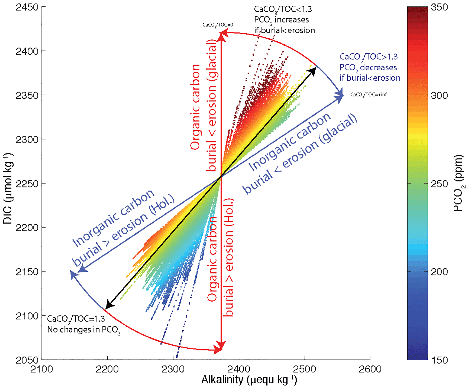
Figure 12Atmospheric PCO2, DIC and alkalinity in the deep ocean for the shelf scenarios (Fig. 8b). Each experiment appears as a straight line of dots and each dot corresponds to a 1 kyr time step. The tilt of the individual scenario lines depends on the CaCO3 : Corg burial ratio in shelf sediments. Blue and red lines correspond to 100 % carbonate and 100 % Corg burial, respectively.
5.4 Implications of geological fluxes for whole-ocean δ13C and terrestrial biosphere
Because the changes in burial on shelves would have changed the global CaCO3 : Corg burial, they must have left a signature in the δ13C of the active carbon inventory, with a strong likelihood for lower δ13C during MIS3–MIS2. This isotopic effect arises from the fact that Corg burial (which removes carbon with very low δ13C) is strongly focused on continental margins, compared to carbonate burial, which is more evenly distributed between margins and the deep sea. Higher Corg burial in the deep sea during glacial maxima (Cartapanis et al., 2016) was insufficient to compensate for reduced burial on shelves. The smaller proportion of low δ13Corg buried during periods of low sea level would have produced a downward drift of the δ13C of the active carbon inventory (Wallmann et al., 2016), while enhanced volcanic activity could have reduced δ13C during deglaciation (Huybers and Langmuir, 2009; Roth and Joos, 2012).
This result, previously identified by Wallmann (2016), is important given the frequently applied technique of calculating changes in the terrestrial biosphere using reconstructed changes in whole-ocean δ13C and assuming a constant inventory (Shackleton, 1977; Bird et al., 1996; Ciais et al., 2012; Menviel et al., 2012; Peterson et al., 2014; Schmittner and Somes, 2016). The magnitude of ocean δ13C changes that result from changes in shelf burial is highly uncertain, given the large range in estimated modern burial fluxes, but could potentially exceed the observed glacial–interglacial change of 0.32 ‰ (Wallmann et al., 2016). Unfortunately, this invalidates the use of δ13C as a direct monitor of changes in the terrestrial biosphere, and requires that new types of constraints on changes in terrestrial biosphere be developed.
Although the uncertainties are large, our mass-balance calculations suggest that the terrestrial biosphere during the LGM was most likely larger than implied by the constant-inventory assumption. We note that using the highest modern Corg burial flux (on the order of 500 PgC kyr−1) would imply a change of the δ13C of the system on the order of 1 ‰ (Figs. 8 and 10), which is higher than reconstructed variability for δ13C in the deep ocean, in which most of the carbon resides (Oliver et al., 2010; Peterson et al., 2014). This suggests that either the highest estimates for modern burial over shelves (above 500 PgC kyr−1) are inconsistent with the assumption of a 60 % decrease of the shelf burial during peak glacial or that the terrestrial biosphere actually contained more biomass during the glacial than today, in contrast to the standard assumption. Although this is highly uncertain, such a change could have occurred through an expansion of peatlands and permafrost carbon during the glacial (Ciais et al., 2012). An expansion of terrestrial carbon storage in a colder state would perhaps be more consistent with the general expectation for carbon release from peatland and permafrost under anthropogenic warming (IPCC, 2014), though it should be viewed as a highly speculative possibility.
5.5 Non-steady-state Holocene carbon cycle
Our results show that the removal rate of carbon from the active pool was higher during the Holocene (prior to anthropogenic carbon release) compared to the glacial (Fig. 10c). This result, which emerges primarily from the fact that CaCO3 burial, both on the shelves and in the deep sea, was faster than it had been during the glacial, indicates that the active carbon inventory was shrinking prior to anthropogenic inputs. The estimates suggest that this imbalance was mostly attributable to the shelf burial, though at a rate that was very slow compared to subsequent fossil fuel emissions (∼100 PgC kyr−1 net loss vs. present-day emissions of ∼10 000 PgC kyr−1).
In support of this large glacial–interglacial variation in carbon burial rates, we find that only mass-balance calculations that include reduced burial during the glacial infer background inputs of carbon that are consistent with the <400 PgC kyr−1 geological inputs estimated in the literature (Fig. 1). Essentially, without slower burial during the glacial, modern-day burial estimates would require larger carbon input fluxes than supported by observational estimates in order to balance the long-term inventory. Although this consistency does not amount to proof, it provides encouraging support for the emergent picture of a geological carbon cycle that is dynamic on the timescale of glacial cycles.
We have made use of an extensive, quality-controlled database for marine sedimentary proxies, to present the first global quantitative reconstruction of carbon and alkalinity burial in deep-sea sediments over the last glacial cycle. Our reconstructions of carbonate and Corg burial in the deep ocean provide the first dynamic estimate of these major components of carbon removal over a full glacial cycle.
Our reconstruction indicates that CaCO3 removal fluxes in deep-sea sediment remained indistinguishable from the Holocene during MIS5, dropped to their lowest value during MIS4 (78 % ± 9 % of Holocene value), and remained lower than the Holocene during MIS2 (85 % ± 7 %). The reduction of carbonate burial in the Atlantic Ocean during the glacial was not entirely compensated by increased burial in the Pacific Ocean, implying the buildup of alkalinity in the glacial ocean (given the assumption that the alkalinity supply from weathering remained constant). We suggest that this weak compensation of burial was primarily related to the parallel accumulation of DIC in the deep sea, which counteracted the alkalinity buildup to prevent high [] in deep water. Moreover, the reduction of shelf burial during sea level lowstands would have unquestionably grown the active carbon and oceanic alkalinity inventories, followed by reduction of the inventories when sea level rose and rapid shelf burial resumed. The consequent changes in the global ratio of CaCO3 : Corg burial would have produced significant changes in the δ13C of the active carbon pool, invalidating the simple use of whole-ocean δ13C to reconstruct changes in the terrestrial biosphere.
The emergent picture of these results suggests that geological carbon fluxes are more dynamic than frequently assumed and that this includes not just the input fluxes but also the output fluxes through marine burial. Our reconstruction implies that the Holocene C cycle was significantly out of balance. As a result, these fluxes need to be considered as an integral part of glacial–interglacial cycles.
Results and references used can be accessed in the Supplement.
Our reconstructions are affected by multiple sources of uncertainty. We identify four different types of uncertainty in Sect. A and indicate whether each error is expected to be independent of the others. We then estimate the contributions from the most important sources of uncertainty using bootstrap analyses (see Sect. B).
A1 Uncertainty in the sedimentary records
First, there is some uncertainty associated with the quantification of past changes in the CaCO3 accumulation rate in each downcore record. This can be further subdivided into three uncertainties:
- a.
Measurement of CaCO3 concentration. This has an analytical error order of 3 %; it is independent.
- b.
Linear sediment accumulation rate. This is potentially large over periods less than age control point spacing but small (a few percent) when integrated over the span of multiple age control points; it is independent.
- c.
Sediment density. Based on the literature, and using our database, we attempted to understand the relationships between depth in the sediment, sediment composition, and sediment density. The density of the sediment is partly dependent on the carbonate content, but carbonate content influence on the density depends also on the density of the other components of the sediment (Reghellin et al., 2013), so that it was not possible to accurately infer density variations from the changes in the carbonate content alone. Attempts to estimate density from other sedimentary variables based on existing calibrations (Dadey et al., 1992; Weber et al., 1997; Fortin et al., 2013) were not successful. Unassessed changes of sediment density are therefore likely to introduce uncertainty for many records, although the largest and most systematic change is likely to be the long-term increasing trend caused by compaction, which is addressed by the long-term trend correction. This source of uncertainties is mostly independent, though it could possibly correlate with CaCO3 content.
We assume that these errors are small (probably less than 10 % relative error) and uncorrelated with the other larger sources of error given below and therefore do not formally assess them.
A2 Representativity of local regions by sedimentary records
Each downcore record may be biased relatively to its surrounding environment. Many paleoceanographic cores are purposefully collected from rapidly accumulating sites in order to maximize temporal resolution. This intentional collection bias towards high sedimentation rate sites could affect the representativity of the following:
- a.
CaCO3 concentration due to differential transport and/or preservation of CaCO3. The magnitude is unknown, though the fact that paleoceanographers very frequently use high accumulation rate sites in order to infer regional changes in sediment composition implies that it is generally thought to be minor. It is possibly correlated with point (b) in Sect. A2 through differential transport of CaCO3 vs. other sediment fractions.
- b.
Mass accumulation rate, if the accumulation rate in the cored location varies in a way that is not proportional to variation of sedimentation rates in the local region. The magnitude is unknown but presumably large for some very rapidly accumulating “drift” sites where sediment focus changes over time. These changes will cancel each other out to some degree if multiple cores in the same region are considered, since a relative decrease in sedimentation rate at one site must be compensated by a relative increase elsewhere, although there is no guarantee that the available sampling density is sufficient to achieve this. It is possibly correlated with point (a) in Sect. A2.
The uncertain representativity at the local scale (including both points (a) and (b) in Sect. A2) is addressed by bootstrap resampling of the available sedimentary records (see Sect. A4 and Fig. A2).
A3 Province maps
In order to account for spatial coherence in the geographic and bathymetric variability in global carbonate burial, we subdivided the world ocean into contiguous regions we refer to “provinces”. As any subdivision will introduce inherent bias, we used a total of 20 different province maps, allowing us to analyze the dependency of our results on the province map used (Fig. A1). The first two maps simply subdivide the world ocean into major ocean basins (map 1), as well as a finer subdivision into seas based on the International Hydrographic Organization (1953) definition (map 3). Because carbonate export from the ocean surface largely depends on the biogeochemical conditions at the surface, we also used the annual climatology of the ocean biogeochemical provinces based on (Longhurst, 1995), recently updated by Reygondeau et al. (2013) (map 4). This map distinguishes 56 coherent provinces from a biogeochemical perspective. We simplified and adapted this map to match our sample distribution and came up with two sets of maps subdivided in 15 and 30 provinces, respectively (maps 5 and 7). Water depth is also important for carbonate, given that carbonate solubility varies as a direct result of pressure. In order to resolve the possible influence of depth on our reconstruction, we separated the two modified Longhurst maps into a shallow and deep component, following the 1500 m isobaths (maps 6 and 8). Furthermore, given the potential importance of changes in carbonate preservation due to changes of water column chemistry, we subdivided the ocean according to the carbonate saturation state at ocean bottom (Ωcal<0.8; 0.8<Ωcal<1.2; Ωcal>1.2) (Dunne et al., 2012) (map 2). Finally, in order to account for the potential heterogeneity close to coasts, we subdivided the ocean map, the sea map, and the two simplified Longhurst maps into coastal and open ocean provinces, using three different thresholds of distance from the closest shoreline: 500, 1000, and 1500 km (maps 9 to 20; see details of the results for individual province maps in Figs. A2, A4, and A5).

Figure A1Province maps used in this study; see details in the text. 1. ocean; 2. carbonate saturation; 3. seas; 4. Longhurst; 5. simplified Longhurst 1 (S.L.1). 6. S.L.1 plus depth; 7. S.L.2; 8. S.L.2 plus depth; 9. ocean 500 km; 10. ocean 1000 km; 11. ocean 1500 km; 12. S.L.1 500 km; 13. S.L.1 1000 km; 14. S.L.1 1500 km; 15. S.L.2 500 km; 16. S.L.2 1000 km; 17. S.L.2 1500 km; 18. seas 500 km; 19. seas 1000 km; 20. seas 1500 km.
A4 Heterogeneity within provinces
As discussed above, sediment cores represent local regions within provinces. Temporal trends in the burial flux of CaCO3 within any given local region will differ, to some degree, from the trend of the larger province in which the region is located. The larger the province, the more severe this problem is likely to be. This heterogeneity is alleviated, to some degree, by averaging multiple records within a given province (Fig. A1).
It is important to consider that there may be a systematic bias, given that cores tend to be located in the most rapidly accumulating regions of provinces, including continental slopes. However, although this would lead to incorrect inferences regarding changes in CaCO3 MAR in the slowly accumulating regions of the province, it is less of a problem for estimating the total CaCO3 MAR within the province, given that the rapidly accumulating regions are more important for the overall burial flux, and therefore it is most important that they be well constrained.
The heterogeneity uncertainty is independent of the others and is addressed by the bootstrap resampling across multiple configurations of the province maps (Sect. B).

Figure A2Illustrative summary figure for the province map S.L.2. Panel (a) shows relative changes in downcore CaCO3 MAR (ln(LGM/Holocene)) in each province. Box plot shows 0 % (bottom whiskers), 25 %, 50 % (median; red lines), 75 %, and 100 % (top whiskers) quantiles, as well as mean (green cross) and outliers (red cross), for each province. Panel (b) shows the contribution by province to modern CaCO3 MAR, in descending order (blue curve) and the number of records used in each province (green). Panel (c) shows the history of absolute changes in CaCO3 MAR for the last 150 kyr, based on the bootstrap experiment (5th, 25th, 75th, and 95th percentile ranges are shaded, and the bootstrap mean plotted in red) compared to the calculation using all available records (black). Panel (d) shows the temporal variations in coverage based on the bootstrap experiment. The 5th, 25th, 75th, and 95th percentiles are shaded, and the bootstrap mean is plotted in red. The black dotted line corresponds to the coverage variations using all available records.
A5 Uncertainty in map reconstructions
Inaccuracy in the spatial distribution of CaCO3 burial in the modern map reconstruction will incorrectly weight the relative changes in different provinces in calculating the global burial flux. This uncertainty is independent of the others.
We discussed this aspect above (Fig. A2 and Table 1) and include it in the bootstrap below by repeating the calculations with the two available maps. Given that the two maps are constrained with the same data, this is likely an underestimate of the true uncertainty. In the future, this could be revisited when new data-constrained maps of CaCO3 burial flux become available. Nonetheless, our results indicate very similar temporal patterns for the two modern maps used, suggesting that our reconstruction is relatively insensitive to this uncertainty (Table 1). Given that this uncertainty is independent of the others, it is not likely to be highly significant for the final outcome.
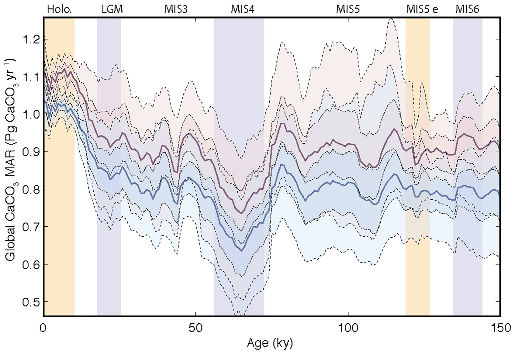
Figure A3Global carbonate burial using two different modern MAR maps. Lines and shaded areas show the reconstructed time histories of global carbonate burial using a modern carbonate MAR map based on sedimentary data (red) and on a metamodel tuned to fit the sedimentary data (blue); see also Fig. 2. The distribution shown by dotted lines and shaded areas (5th, 25th, 50th, 75th, and 95th percentiles) was calculated from a bootstrap experiment performed on the 20 province maps used in the study.
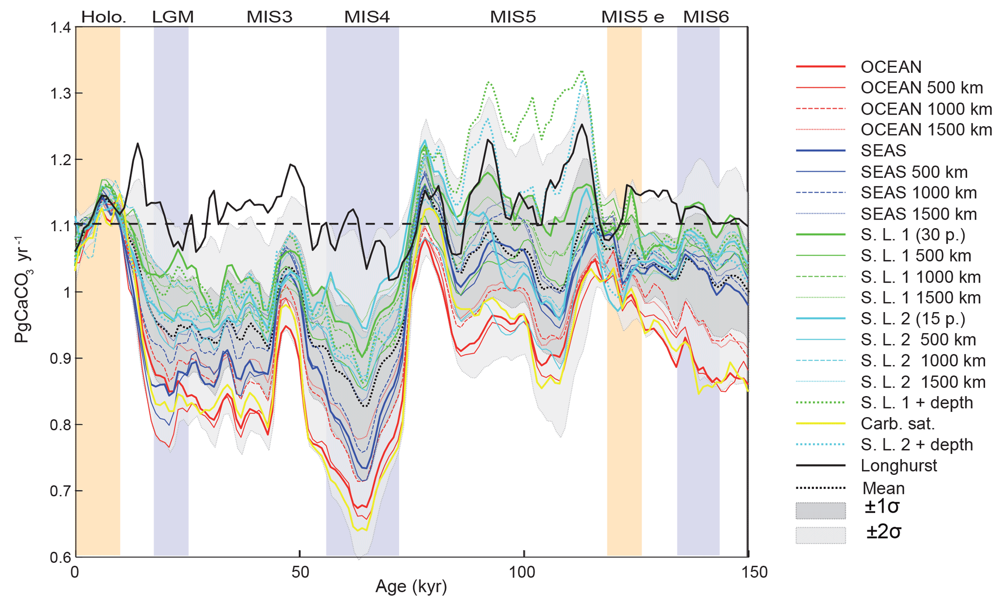
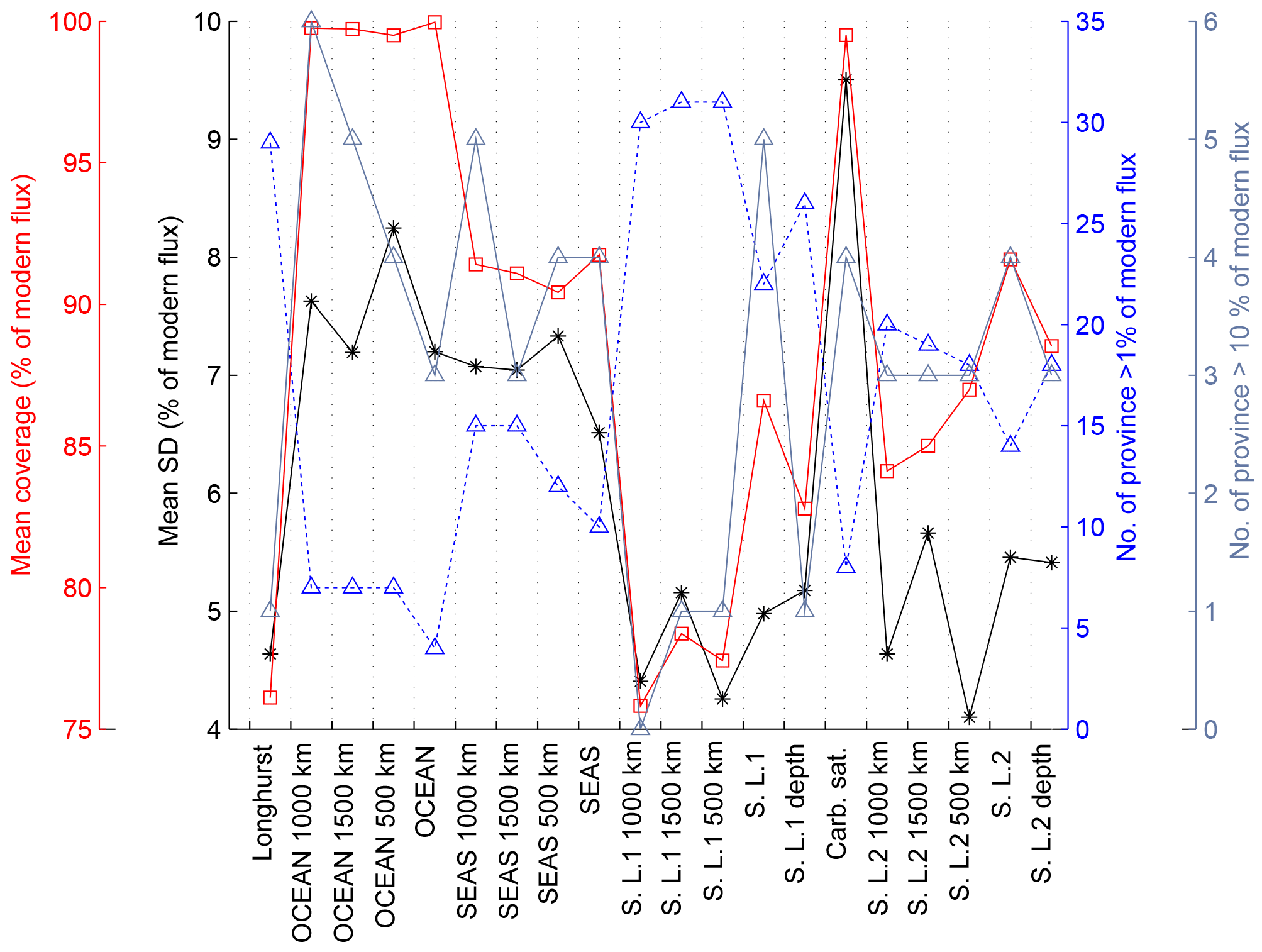
Figure A5Summary of province-map experiments. Black symbols show the mean of the standard deviation at each time step of the bootstrap experiment for each province map. Red symbols show the mean coverage for the bootstrap experiment for each province map. The number of provinces accounting for more than 1 % and 10 % of the modern flux for each province map are shown by the blue and grey symbols, respectively.
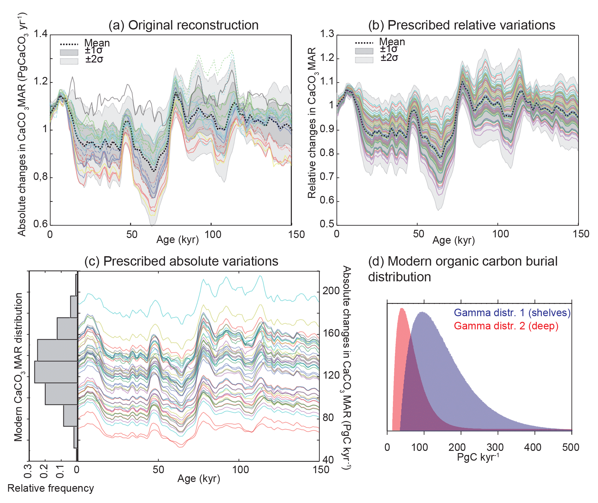
Figure A6Construction of time series for scenarios. (a) Original reconstruction from the 20 province-map scenarios. (b) Prescribed relative variations derived from the distribution in panel (a). (c) Prescribed absolute variations derived from the product of (b) and the assigned modern burial distribution (see details in Table 3). (d) Prescribed modern Corg burial distribution over shelf (gamma distribution of 1, mean of 160; median of 140; mode of 100; SD of 80) and permanently submerged deep-sea environments (gamma distribution of 2, mean of 70; median of 60; mode of 40; SD of 40).
In order to quantitatively estimate the impact of uncertainties itemized above on our reconstruction, we performed a series of bootstrap experiments and the 20-province-map set. Each experiment consisted of repeating the entire calculation for each province map by randomly selecting n records out of the n available records in each province, allowing a single record to be selected multiple times. Each record was expressed as the relative deviation over time from the mean Holocene value. The geometric mean of the new set of n time series was subsequently multiplied by modern MAR in the province, at each time step. For any time period in which no downcore records were available within a province, the MAR for that province was set at the modern value. The coverage was calculated at each time step as the sum of the modern MAR for provinces where downcore records were available, divided by the global modern MAR. This operation was repeated 10 000 times for each province map.
We also tested the influence of the modern MAR map by using the two modern MAR maps shown in Fig. 2. These two maps have different absolute modern CaCO3 MARs and also distribute the modern MAR differently among provinces (Table 1), allowing a test of the robustness of our method to different modern MAR distributions (Fig. A3). The relative changes in our reconstructed global carbonate burial over time do not depend on the choice of maps, as shown in Fig. A3.
The results of the bootstrap experiment for each province map, using modern map 1, are shown in Fig. A3, and a summary of the results is displayed in Fig. A3. It is important to keep in mind that the coverage calculated here can only be equal to or lower than the normal calculation using all records, due to bootstrap resampling (Fig. A2d).
The province-map scenarios that result in the lowest amplitude during MIS2 and MIS4 are also the ones that have the lowest coverage, as a higher proportion of the total burial is set as constant for these maps (see Table 2, Fig. A5). This effect also explains the lower amplitude affecting MIS6–MIS5 transition as compared to MIS2–MIS1. Using the mean and the standard deviation of the 20 province-map scenarios, which do not cover exactly the same surfaces, tends to decrease the variability of the mean curve, while increasing the standard deviation such as the final distribution of the burial is rather conservative.
Although we could use these bootstrap reconstructions to provide a mean and standard deviation of the forcings, we instead use the time series using all available records, in order to make as complete use as possible of the available data. Given that the individual province-map scenarios are distributed quite symmetrically around the mean scenario (Figs. A4 and A6), we used the relative changes in the mean reconstruction as shown in Fig. A6a, to which we add, at each time step, a normally distributed fraction of the relative standard deviations calculated from the 20 province-map scenarios. Note that the mean standard deviation used here (equal to the mean of the mean standard deviation calculated from the 20 province-map scenarios at each time step, equivalent to approximately 7 % of the modern global burial flux) is in the higher range of the mean standard deviation calculated from the bootstrap experiment for each province map (Fig. A5). Thus, although we do not use the bootstrap results here directly, they are consistent with the uncertainty range applied. The time series are prescribed as variations relative to the modern global burial flux (Fig. A6b and c).
The supplement related to this article is available online at: https://doi.org/10.5194/cp-14-1819-2018-supplement.
OC, DB and EDG designed the proxy database and the data analysis. OC performed the analyses. OC, DB, EDG and SLJ wrote the manuscript. All authors contributed to the interpretation of the results.
The authors declare that they have no conflict of interest.
Olivier Cartapanis and Samuel L. Jaccard were funded by the Swiss National Science Foundation (grants
PP00P2-144811 and PP00P2_172915). Olivier Cartapanis and Daniele Bianchi were funded
by the Canadian Institute for Advanced Research (CIFAR). Eric D. Galbraith acknowledges
financial support from the Spanish Ministry of Economy and Competitiveness,
through the María de Maeztu Programme for Centres/Units of Excellence
in R&D (MDM-2015-0552). The author would like to thank editor Luke Skinner,
anonymous referees, and Andreas Schmittner for their valuable comments and
suggestions that greatly improved the quality of the paper.
Edited by: Luke Skinner
Reviewed by: Andreas Schmittner and one anonymous referee
Amante, C. and Eakins, B. W.: ETOPO1 1 arc-minute global relief model: procedures, data sources and analysis, US Department of Commerce, National Oceanic and Atmospheric Administration, National Environmental Satellite, Data, and Information Service, National Geophysical Data Center, Marine Geology and Geophysics Division Colorado, 2009.
Amiotte Suchet, P., Probst, J.-L., and Ludwig, W.: Worldwide distribution of continental rock lithology: Implications for the atmospheric/soil CO2 uptake by continental weathering and alkalinity river transport to the oceans, Global Biogeochem. Cy., 17, 1038, https://doi.org/10.1029/2002GB001891, 2003.
Archer, D., Winguth, A., Lea, D., and Mahowald, N.: What caused the glacial/interglacial atmospheric pCO2 cycles?, Rev. Geophys., 38, 159–189, https://doi.org/10.1029/1999rg000066, 2000.
Bauer, J. E., Cai, W.-J., Raymond, P. A., Bianchi, T. S., Hopkinson, C. S., and Regnier, P. A. G.: The changing carbon cycle of the coastal ocean, Nature, 504, 61–70, https://doi.org/10.1038/nature12857, 2013.
Berelson, W. M., Balch, W. M., Najjar, R., Feely, R. A., Sabine, C., and Lee, K.: Relating estimates of CaCO3 production, export, and dissolution in the water column to measurements of CaCO3 rain into sediment traps and dissolution on the sea floor: A revised global carbonate budget, Global Biogeochem. Cy., 21, gb1024, https://doi.org/10.1029/2006gb002803, 2007.
Berger, W. H.: Increase of carbon dioxide in the atmosphere during deglaciation: the coral reef hypothesis, Naturwissenschaften, 69, 87–88, https://doi.org/10.1007/BF00441228, 1982.
Berner, R. A.: The Long Term Stability of the Earth System Biogeochemical cycles of carbon and sulfur and their effect on atmospheric oxygen over phanerozoic time, Palaeogeogr. Palaeocl., 75, 97–122, https://doi.org/10.1016/0031-0182(89)90186-7, 1989.
Bird, M. I., Llyod, J., and Farquhar, G. D.: Terrestrial carbon-storage from the Last Glacial Maximum to the present, Chemosphere, 33, 1675–1685, 1996.
Boyle, E. A.: Vertical oceanic nutrient fractionation and glacial/interglacial CO2 cycles, Nature, 331, 55–56, 1988.
Boyle, E. A. and Keigwin, L. D.: Deep circulation of the North Atlantic over the last 200 000 years: Geochemical evidence, Science, 218, 784–787, 1982.
Broecker, W. S.: Ocean chemistry during glacial time, Geochim. Cosmochim. Acta, 46, 1689–1705, https://doi.org/10.1016/0016-7037(82)90110-7, 1982.
Broecker, W. S. and Peng, T. H.: The oceanic salt pump: Does it contribute to the glacial-interglacial difference in atmospheric CO2 content?, Global Biogeochem. Cy., 1, 251–259, https://doi.org/10.1029/GB001i003p00251, 1987.
Brzezinski, M. A., Pride, C. J., Franck, V. M., Sigman, D. M., Sarmiento, J. L., Matsumoto, K., Gruber, N., Rau, G. H., and Coale, K. H.: A switch from Si(OH)4 to depletion in the glacial Southern Ocean, Geophys. Res. Lett., 29, 1564, https://doi.org/10.1029/2001gl014349, 2002.
Burdige, D. J.: Burial of terrestrial organic matter in marine sediments: A re-assessment, Global Biogeochem. Cy., 19, GB4011, https://doi.org/10.1029/2004GB002368, 2005.
Burdige, D. J.: Preservation of Organic Matter in Marine Sediments: Controls, Mechanisms, and an Imbalance in Sediment Organic Carbon Budgets?, Chem. Rev., 107, 467–485, https://doi.org/10.1021/cr050347q, 2007.
Burton, M. R., Sawyer, G. M., and Granieri, D.: Deep carbon emissions from volcanoes, Rev. Mineral. Geochem, 75, 323–354, 2013.
Cartapanis, O., Bianchi, D., Jaccard, S. L., and Galbraith, E. D.: Global pulses of organic carbon burial in deep-sea sediments during glacial maxima, Nat. Commun., 7, 10796, https://doi.org/10.1038/ncomms10796, 2016.
Cartigny, P., Jendrzejewski, N., Pineau, F., Petit, E., and Javoy, M.: Volatile (C, N, Ar) variability in MORB and the respective roles of mantle source heterogeneity and degassing: the case of the Southwest Indian Ridge, Earth Planet. Sc. Lett., 194, 241–257, https://doi.org/10.1016/S0012-821X(01)00540-4, 2001.
Catubig, N. R., Archer, D. E., Francois, R., deMenocal, P., Howard, W., and Yu, E. F.: Global deep-sea burial rate of calcium carbonate during the last glacial maximum, Paleoceanography, 13, 298–310, https://doi.org/10.1029/98pa00609, 1998.
Chavrit, D., Humler, E., and Grasset, O.: Mapping modern CO2 fluxes and mantle carbon content all along the mid-ocean ridge system, Earth Planet. Sc. Lett., 387, 229–239, https://doi.org/10.1016/j.epsl.2013.11.036, 2014.
Ciais, P., Tagliabue, A., Cuntz, M., Bopp, L., Scholze, M., Hoffmann, G., Lourantou, A., Harrison, S. P., Prentice, I. C., Kelley, D. I., Koven, C., and Piao, S. L.: Large inert carbon pool in the terrestrial biosphere during the Last Glacial Maximum, Nat. Geosci., 5, 74–79, 2012.
Coltice, N., Simon, L., and Lécuyer, C.: Carbon isotope cycle and mantle structure, Geophys. Res. Lett., 31, L05603, https://doi.org/10.1029/2003GL018873, 2004.
Copard, Y., Amiotte-Suchet, P., and Di-Giovanni, C.: Storage and release of fossil organic carbon related to weathering of sedimentary rocks, Earth Planet. Sc. Lett., 258, 345–357, https://doi.org/10.1016/j.epsl.2007.03.048, 2007.
Covault, J. A. and Graham, S. A.: Submarine fans at all sea-level stands: Tectono-morphologic and climatic controls on terrigenous sediment delivery to the deep sea, Geology, 38, 939–942, https://doi.org/10.1130/g31081.1, 2010.
Curry, W. B., Duplessy, J.-C., Labeyrie, L., and Shackleton, N. J.: Changes in the distribution of δ13C of deep water ΣCO2 between the last glaciation and the Holocene, Paleoceanography and Paleoclimatology, 3, 317–341, 1988.
Dadey, K. A., Janecek, T., and Klaus, A.: Dry-bulk density: its use and determination, in: Proc. ODP, Sci. Results, edited by: Taylor, B., Fujioka, K., et al., 126, College Station, TX (Ocean Drilling Program), 551–554. https://doi.org/10.2973/odp.proc.sr.126.157.1992, 1992.
Degens, E. T.: Biogeochemistry of Stable Carbon Isotopes, in: Organic Geochemistry, edited by: Eglinton, G. and Murphy, M. J., Springer, Berlin, Heidelberg, 304–329, 1969.
Deines, P.: The carbon isotope geochemistry of mantle xenoliths, Earth-Sci. Rev., 58, 247–278, https://doi.org/10.1016/S0012-8252(02)00064-8, 2002.
Dickson, A. G. and Goyet, C.: Handbook of methods for the analysis of the various parameters of the carbon dioxide system in sea water, Version 2, San Diego, ORNL/CDIAC-74, 1994.
Dubois, N., Kienast, M., Kienast, S., Calvert, S. E., Francois, R., and Anderson, R. F.: Sedimentary opal records in the eastern equatorial Pacific: It is not all about leakage, Global Biogeochem. Cy., 24, GB4020, https://doi.org/10.1029/2010gb003821, 2010.
Dunne, J. P., Sarmiento, J. L., and Gnanadesikan, A.: A synthesis of global particle export from the surface ocean and cycling through the ocean interior and on the seafloor, Global Biogeochem. Cy., 21, GB4006, https://doi.org/10.1029/2006GB002907, 2007.
Dunne, J. P., Hales, B., and Toggweiler, J. R.: Global calcite cycling constrained by sediment preservation controls, Global Biogeochem. Cy., 26, GB3023, https://doi.org/10.1029/2010GB003935, 2012.
Eggleston, S. and Galbraith, E. D.: The devil's in the disequilibrium: multi-component analysis of dissolved carbon and oxygen changes under a broad range of forcings in a general circulation model, Biogeosciences, 15, 3761–3777, https://doi.org/10.5194/bg-15-3761-2018, 2018.
Farrell, J. W. and Prell, W. L.: Climatic change and CaCO3 preservation: an 800 000 year bathymetric reconstruction from the central equatorial Pacific Ocean, Paleoceanography, 4, 447–466, 1989.
Fortin, D., Francus, P., Gebhardt, A. C., Hahn, A., Kliem, P., Lisé-Pronovost, A., Roychowdhury, R., Labrie, J., and St-Onge, G.: Destructive and non-destructive density determination: method comparison and evaluation from the Laguna Potrok Aike sedimentary record, Quaternary Sci. Rev., 71, 147–153, https://doi.org/10.1016/j.quascirev.2012.08.024, 2013.
Foster, G. L. and Vance, D.: Negligible glacial-interglacial variation in continental chemical weathering rates, Nature, 444, 918–921, 2006.
Freeman, K. H. and Hayes, J. M.: Fractionation of carbon isotopes by phytoplankton and estimates of ancient CO2 levels, Global Biogeochem. Cy., 6, 185–198, https://doi.org/10.1029/92GB00190, 1992.
Gaillardet, J., Dup ré, B., Louvat, P., and Allègre, C. J.: Global silicate weathering and CO2 consumption rates deduced from the chemistry of large rivers, Chem. Geol., 159, 3–30, https://doi.org/10.1016/S0009-2541(99)00031-5, 1999.
Galbraith, E. D. and Jaccard, S. L.: Deglacial weakening of the oceanic soft tissue pump: global constraints from sedimentary nitrogen isotopes and oxygenation proxies, Quaternary Sci. Rev., 109, 38–48, https://doi.org/10.1016/j.quascirev.2014.11.012, 2015.
Galy, V., Peucker-Ehrenbrink, B., and Eglinton, T.: Global carbon export from the terrestrial biosphere controlled by erosion, Nature, 521, 204–207, https://doi.org/10.1038/nature14400, 2015.
Gerlach, T.: Volcanic versus anthropogenic carbon dioxide, Eos, Trans. AGU, 92, 201–202, https://doi.org/10.1029/2011EO240001, 2011.
Gibbs, M. T. and Kump, L. R.: Global chemical erosion during the Last Glacial Maximum and the present: Sensitivity to changes in lithology and hydrology, Paleoceanography, 9, 529–543, https://doi.org/10.1029/94PA01009, 1994.
Grant, K. M., Rohling, E. J., Bar-Matthews, M., Ayalon, A., Medina-Elizalde, M., Ramsey, C. B., Satow, C., and Roberts, A. P.: Rapid coupling between ice volume and polar temperature over the past 150 000 years, Nature, 491, 744–747, https://doi.org/10.1038/nature11593, 2012.
Guihou, A., Pichat, S., Govin, A., Nave, S., Michel, E., Duplessy, J.-C., Telouk, P., and Labeyrie, L.: Enhanced Atlantic Meridional Overturning Circulation supports the Last Glacial Inception, Quaternary Sci. Rev., 30, 1576–1582, 2011.
Hain, M. P., Sigman, D. M., and Haug, G. H.: Carbon dioxide effects of Antarctic stratification, North Atlantic Intermediate Water formation, and subantarctic nutrient drawdown during the last ice age: Diagnosis and synthesis in a geochemical box model, Global Biogeochem. Cy., 24, GB4023, https://doi.org/10.1029/2010GB003790, 2010.
Hain, M. P., Sigman, D. M., and Haug, G. H.: 8.18 – The Biological Pump in the Past, in: Treatise on Geochemistry, Second Edition, edited by: Turekian, H. D. H. and Karl, K., Elsevier, Oxford, 485–517, 2014.
Hartmann, J., Moosdorf, N., Lauerwald, R., Hinderer, M., and West, A. J.: Global chemical weathering and associated P-release – The role of lithology, temperature and soil properties, Chem. Geol., 363, 145–163, https://doi.org/10.1016/j.chemgeo.2013.10.025, 2014.
Hedges, J. I. and Keil, R. G.: Sedimentary organic matter preservation: an assessment and speculative synthesis, Mar. Chem., 49, 81–115, https://doi.org/10.1016/0304-4203(95)00008-F, 1995.
Herman, F., Seward, D., Valla, P. G., Carter, A., Kohn, B., Willett, S. D., and Ehlers, T. A.: Worldwide acceleration of mountain erosion under a cooling climate, Nature, 504, 423–426, https://doi.org/10.1038/nature12877, 2013.
Hoegh-Guldberg, O., Mumby, P. J., Hooten, A. J., Steneck, R. S., Greenfield, P., Gomez, E., Harvell, C. D., Sale, P. F., Edwards, A. J., Caldeira, K., Knowlton, N., Eakin, C. M., Iglesias-Prieto, R., Muthiga, N., Bradbury, R. H., Dubi, A., and Hatziolos, M. E.: Coral Reefs Under Rapid Climate Change and Ocean Acidification, Science, 318, 1737–1742, https://doi.org/10.1126/science.1152509, 2007.
Huybers, P. and Langmuir, C.: Feedback between deglaciation, volcanism, and atmospheric CO2, Earth Planet. Sc. Lett., 286, 479–491, https://doi.org/10.1016/j.epsl.2009.07.014, 2009.
International Hydrographic Organization: Limits of Oceans and Seas, Special Publication, 23, hdl:10013/epic.37175.d001, 1953.
IPCC: Climate Change 2014: Impacts, Adaptation, and Vulnerability, Part A: Global and Sectoral Aspects, Contribution of Working Group II to the Fifth Assessment Report of the Intergovernmental Panel on Climate Change, edited by: Field, C. B., Barros, V. R., Dokken, D. J., Mach, K. J., Mastrandrea, M. D., Bilir, T. E., Chatterjee, M., Ebi, K. L., Estrada, Y. O., Genova, R. C., Girma, B., Kissel, E. S., Levy, A. N., MacCracken, S., Mastrandrea, P. R., and White, L. L., Cambridge University Press, Cambridge, UK and New York, NY, USA, 1132 pp., 2014.
Jaccard, S., Haug, G., Sigman, D., Pedersen, T., Thierstein, H., and Röhl, U.: Glacial/interglacial changes in subarctic North Pacific stratification, Science, 308, 1003–1006, 2005.
Jaccard, S., Hayes, C. T., Martínez-García, A., Hodell, D., Anderson, R. F., Sigman, D., and Haug, G.: Two modes of change in Southern Ocean productivity over the past million years, Science, 339, 1419–1423, 2013.
Jaccard, S. L., Galbraith, E. D., Sigman, D. M., Haug, G. H., Francois, R., Pedersen, T. F., Dulski, P., and Thierstein, H. R.: Subarctic Pacific evidence for a glacial deepening of the oceanic respired carbon pool, Earth Planet. Sc. Lett., 277, 156–165, https://doi.org/10.1016/j.epsl.2008.10.017, 2009.
Jahnke, R. A.: The global ocean flux of particulate organic carbon: Areal distribution and magnitude, Global Biogeochem. Cy., 10, 71–88, https://doi.org/10.1029/95GB03525, 1996.
Jellinek, A. M., Manga, M., and Saar, M. O.: Did melting glaciers cause volcanic eruptions in eastern California? Probing the mechanics of dike formation, J. Geophys. Res.-Sol. Ea., 109, B09206, https://doi.org/10.1029/2004JB002978, 2004.
Keil, R.: Anthropogenic Forcing of Carbonate and Organic Carbon Preservation in Marine Sediments, Annu. Rev. Mar. Sci., 9, 151–172, https://doi.org/10.1146/annurev-marine-010816-060724, 2017.
Kohfeld, K. E. and Chase, Z.: Temporal evolution of mechanisms controlling ocean carbon uptake during the last glacial cycle, Earth Planet. Sc. Lett., 472, 206–215, https://doi.org/10.1016/j.epsl.2017.05.015, 2017.
Kump, L. R. and Arthur, M. A.: Interpreting carbon-isotope excursions: carbonates and organic matter, Chem. Geol., 161, 181–198, https://doi.org/10.1016/S0009-2541(99)00086-8, 1999.
Kutterolf, S., Jegen, M., Mitrovica, J. X., Kwasnitschka, T., Freundt, A., and Huybers, P. J.: A detection of Milankovitch frequencies in global volcanic activity, Geology, 41, 227–230, https://doi.org/10.1130/g33419.1, 2013.
Labeyrie, L. D., Duplessy, J.-C., Duprat, J., Juillet-Leclerc, A., Moyes, J., Michel, E., Kallel, N., and Shackleton, N. J.: Changes in the vertical structure of the North Atlantic Ocean between glacial and modern times, Quaternary Sci. Rev., 11, 401–413, 1992.
Lambeck, K. and Chappell, J.: Sea Level Change Through the Last Glacial Cycle, Science, 292, 679–686, https://doi.org/10.1126/science.1059549, 2001.
Lee, H., Muirhead, J. D., Fischer, T. P., Ebinger, C. J., Kattenhorn, S. A., Sharp, Z. D., and Kianji, G.: Massive and prolonged deep carbon emissions associated with continental rifting, Nat. Geosci., 9, 145–149, https://doi.org/10.1038/ngeo2622, 2016.
Lisiecki, L. E. and Raymo, M. E.: A Pliocene-Pleistocene stack of 57 globally distributed benthic δ18O records, Paleoceanography, 20, PA1003, https://doi.org/10.1029/2004PA001071, 2005.
Longhurst, A.: Seasonal cycles of pelagic production and consumption, Prog. Oceanogr., 36, 77–167, https://doi.org/10.1016/0079-6611(95)00015-1, 1995.
Lund, D. C., Asimow, P. D., Farley, K. A., Rooney, T. O., Seeley, E., Jackson, E. W., and Durham, Z. M.: Enhanced East Pacific Rise hydrothermal activity during the last two glacial terminations, Science, 351, 478–482, https://doi.org/10.1126/science.aad4296, 2016.
Lynch-Stieglitz, J., Adkins, J. F., Curry, W. B., Dokken, T., Hall, I. R., Herguera, J. C., Hirschi, J. J. M., Ivanova, E. V., Kissel, C., Marchal, O., Marchitto, T. M., McCave, I. N., McManus, J. F., Mulitza, S., Ninnemann, U., Peeters, F., Yu, E. F., and Zahn, R.: Atlantic meridional overturning circulation during the Last Glacial Maximum, Science, 316, 66–69, https://doi.org/10.1126/science.1137127, 2007.
Marchitto, T. M., Lehman, S. J., Ortiz, J. D., Fluckiger, J., and van Geen, A.: Marine radiocarbon evidence for the mechanism of deglacial atmospheric CO2 rise, Science, 316, 1456–1459, https://doi.org/10.1126/science.1138679\textbar ISSN0036-8075, 2007.
Menviel, L., Joos, F., and Ritz, S. P.: Simulating atmospheric CO2, 13C and the marine carbon cycle during the Last Glacial–Interglacial cycle: possible role for a deepening of the mean remineralization depth and an increase in the oceanic nutrient inventory, Quaternary Sci. Rev., 56, 46–68, https://doi.org/10.1016/j.quascirev.2012.09.012, 2012.
Milliman, J. D.: Production and accumulation of calcium carbonate in the ocean: Budget of a nonsteady state, Global Biogeochem. Cy., 7, 927–957, https://doi.org/10.1029/93GB02524, 1993.
Muller-Karger, F. E., Varela, R., Thunell, R., Luerssen, R., Hu, C., and Walsh, J. J.: The importance of continental margins in the global carbon cycle, Geophys. Res. Lett., 32, L01602, https://doi.org/10.1029/2004GL021346, 2005.
Ödalen, M., Nycander, J., Oliver, K. I. C., Brodeau, L., and Ridgwell, A.: The influence of the ocean circulation state on ocean carbon storage and CO2 drawdown potential in an Earth system model, Biogeosciences, 15, 1367–1393, https://doi.org/10.5194/bg-15-1367-2018, 2018.
Oliver, K. I. C., Hoogakker, B. A. A., Crowhurst, S., Henderson, G. M., Rickaby, R. E. M., Edwards, N. R., and Elderfield, H.: A synthesis of marine sediment core δ13C data over the last 150 000 years, Clim. Past, 6, 645–673, https://doi.org/10.5194/cp-6-645-2010, 2010.
Omta, A. W., van Voorn, G. A. K., Rickaby, R. E. M., and Follows, M. J.: On the potential role of marine calcifiers in glacial-interglacial dynamics, Global Biogeochem. Cy., 27, 692–704, https://doi.org/10.1002/gbc.20060, 2013.
Opdyke, B. N. and Walker, J. C. G.: Return of the coral reef hypothesis: Basin to shelf partitioning of CaCO3 and its effect on atmospheric CO2, Geology, 20, 733–736, https://doi.org/10.1130/0091-7613(1992)020<0733:rotcrh>2.3.co;2, 1992.
Orr, J. C., Fabry, V. J., Aumont, O., Bopp, L., Doney, S. C., Feely, R. A., Gnanadesikan, A., Gruber, N., Ishida, A., Joos, F., Key, R. M., Lindsay, K., Maier-Reimer, E., Matear, R., Monfray, P., Mouchet, A., Najjar, R. G., Plattner, G.-K., Rodgers, K. B., Sabine, C. L., Sarmiento, J. L., Schlitzer, R., Slater, R. D., Totterdell, I. J., Weirig, M.-F., Yamanaka, Y., and Yool, A.: Anthropogenic ocean acidification over the twenty-first century and its impact on calcifying organisms, Nature, 437, 681–686, https://doi.org/10.1038/nature04095, 2005.
Peterson, C. D., Lisiecki, L. E., and Stern, J. V.: Deglacial whole-ocean δ13C change estimated from 480 benthic foraminiferal records, Paleoceanography, 29, 549–563, https://doi.org/10.1002/2013PA002552, 2014.
Petsch, S. T.: 12.8 – Weathering of Organic Carbon A2 – Holland, Heinrich D., in: Treatise on Geochemistry, Second Edition, edited by: Turekian, K. K., Elsevier, Oxford, 217–238, 2014.
Reghellin, D., Dickens, G. R., and Backman, J.: The relationship between wet bulk density and carbonate content in sediments from the Eastern Equatorial Pacific, Mar. Geol., 344, 41–52, https://doi.org/10.1016/j.margeo.2013.07.007, 2013.
Reygondeau, G., Longhurst, A., Martinez, E., Beaugrand, G., Antoine, D., and Maury, O.: Dynamic biogeochemical provinces in the global ocean, Global Biogeochem. Cy., 27, 1046–1058, https://doi.org/10.1002/gbc.20089, 2013.
Rickaby, R. E. M., Elderfield, H., Roberts, N., Hillenbrand, C. D., and Mackensen, A.: Evidence for elevated alkalinity in the glacial Southern Ocean, Paleoceanography, 25, PA1209, https://doi.org/10.1029/2009PA001762, 2010.
Ronge, T. A., Tiedemann, R., Lamy, F., Kohler, P., Alloway, B. V., De Pol-Holz, R., Pahnke, K., Southon, J., and Wacker, L.: Radiocarbon constraints on the extent and evolution of the South Pacific glacial carbon pool, Nat. Commun., 7, 11487, https://doi.org/10.1038/ncomms11487, 2016.
Roth, R. and Joos, F.: Model limits on the role of volcanic carbon emissions in regulating glacial–interglacial CO2 variations, Earth Planet. Sc. Lett., 329–330, 141–149, https://doi.org/10.1016/j.epsl.2012.02.019, 2012.
Ryan, D. A., Opdyke, B. N., and Jell, J. S.: Holocene sediments of Wistari Reef: towards a global quantification of coral reef related neritic sedimentation in the Holocene, Palaeogeogr. Palaeocl., 175, 173–184, https://doi.org/10.1016/S0031-0182(01)00370-4, 2001.
Sarmiento, J. L. and Toggweiler, J. R.: A new model for the role of the oceans in determining atmospheric PCO2, Nature, 308, 621–624, 1984.
Sarmiento, J. L. and Gruber, N.: Ocean Biogeochemical Dynamics, Princeton University Press, Princeton, New Jersey, USA, 2006.
Sarmiento, J. L., Dunne, J., Gnanadesikan, A., Key, R. M., Matsumoto, K., and Slater, R.: A new estimate of the CaCO3 to organic carbon export ratio, Global Biogeochem. Cy., 16, 1107, https://doi.org/10.1029/2002gb001919, 2002.
Schmittner, A. and Somes, C.: Complementary Constraints from Carbon (13C) and Nitrogen (15N) Isotopes on the Glacial Ocean's Soft-Tissue Biological Pump, Paleoceanography, 31, 669–693, https://doi.org/10.1002/2015PA002905.
Schumer, R. and Jerolmack, D. J.: Real and apparent changes in sediment deposition rates through time, J. Geophys. Res.-Earth, 114, F00A06, https://doi.org/10.1029/2009JF001266, 2009.
Seiter, K., Hensen, C., Schröter, J., and Zabel, M.: Organic carbon content in surface sediments–defining regional provinces, Deep-Sea Res. Pt. I, 51, 2001–2026, https://doi.org/10.1016/j.dsr.2004.06.014, 2004.
Shackleton, N. J.: Carbon-13 in Uvigerina: Tropical rain forest history and the equatorial Pacific carbonate dissolution cycle, The fate of fossil fuel CO2 in the oceans, New York (Plenum), 401–428, 1977.
Sigman, D. M. and Boyle, E. A.: Glacial/interglacial variations in atmospheric carbon dioxide, Nature, 407, 859–869, 2000.
Sigman, D. M. and Haug, G. H.: 6.18 – The Biological Pump in the Past, in: Treatise on Geochemistry, edited by: Heinrich, D. H. and Karl, K. T., Pergamon, Oxford, 491–528, 2003.
Stott, L., Southon, J., Timmermann, A., and Koutavas, A.: Radiocarbon age anomaly at intermediate water depth in the Pacific Ocean during the last deglaciation, Paleoceanography, 24, PA2223, https://doi.org/10.1029/2008pa001690, 2009.
Sun, X. and Turchyn, A. V.: Significant contribution of authigenic carbonate to marine carbon burial, Nat. Geosci., 7, 201–204, https://doi.org/10.1038/ngeo2070, 2014.
Sundquist, E. T. and Visser, K.: 8.09 – The Geologic History of the Carbon Cycle, in: Treatise on Geochemistry, edited by: Holland, H. D. and Turekian, K. K., Pergamon, Oxford, 425–472, 2003.
Toggweiler, J. R.: Variation of atmospheric CO2 by ventilation of the ocean's deepest water, Paleoceanography, 14, 571–588, https://doi.org/10.1029/1999PA900033, 1999.
Torres, M. A., Moosdorf, N., Hartmann, J., Adkins, J. F., and West, A. J.: Glacial weathering, sulfide oxidation, and global carbon cycle feedbacks, P. Natl. Acad. Sci. USA, 144, 8716–8721, https://doi.org/10.1073/pnas.1702953114, 2017.
Vance, D., Teagle, D. A. H., and Foster, G. L.: Variable Quaternary chemical weathering fluxes and imbalances in marine geochemical budgets, Nature, 458, 493–496, 2009.
Vecsei, A. and Berger, W. H.: Increase of atmospheric CO2 during deglaciation: Constraints on the coral reef hypothesis from patterns of deposition, Global Biogeochem. Cy., 18, GB1035, https://doi.org/10.1029/2003GB002147, 2004.
von Blanckenburg, F., Bouchez, J., Ibarra, D. E., and Maher, K.: Stable runoff and weathering fluxes into the oceans over Quaternary climate cycles, Nat. Geosci., 8, 538–542, https://doi.org/10.1038/ngeo2452, 2015.
Waelbroeck, C., Labeyrie, L., Michel, E., Duplessy, J. C., McManus, J. F., Lambeck, K., Balbon, E., and Labracherie, M.: Sea-level and deep water temperature changes derived from benthic foraminifera isotopic records, Quaternary Sci. Rev., 21, 295–305, 2002.
Wallmann, K., Schneider, B., and Sarnthein, M.: Effects of eustatic sea-level change, ocean dynamics, and nutrient utilization on atmospheric pCO2 and seawater composition over the last 130 000 years: a model study, Clim. Past, 12, 339–375, https://doi.org/10.5194/cp-12-339-2016, 2016.
Wang, X.-C. and Druffel, E. R. M.: Radiocarbon and stable carbon isotope compositions of organic compound classes in sediments from the NE Pacific and Southern Oceans, Mar. Chem., 73, 65–81, https://doi.org/10.1016/S0304-4203(00)00090-6, 2001.
Weber, M. E., Niessen, F., Kuhn, G., and Wiedicke, M.: Calibration and application of marine sedimentary physical properties using a multi-sensor core logger, Mar. Geol., 136, 151–172, 1997.
Yu, J., Broecker, W. S., Elderfield, H., Jin, Z., McManus, J., and Zhang, F.: Loss of Carbon from the Deep Sea Since the Last Glacial Maximum, Science, 330, 1084–1087, 2010.
Yu, J., Anderson, R. F., Jin, Z., Rae, J. W. B., Opdyke, B. N., and Eggins, S. M.: Responses of the deep ocean carbonate system to carbon reorganization during the Last Glacial–interglacial cycle, Quaternary Sci. Rev., 76, 39–52, https://doi.org/10.1016/j.quascirev.2013.06.020, 2013.
Yu, J., Anderson, R. F., and Rohling, E. J.: Deep Ocean Carbonate Chemistry and Glacial-Interglacial Atmospheric CO2 Changes, Oceanography, 27, 16–25, https://doi.org/10.5670/oceanog.2014.04, 2014.
Zech, R.: A permafrost glacial hypothesis – Permafrost carbon might help explaining the Pleistocene ice ages, Quaternary Science Journal, 61, 84–92, 2012.
Zeebe, R. E. and Caldeira, K.: Close mass balance of long-term carbon fluxes from ice-core CO2 and ocean chemistry records, Nat. Geosci., 1, 312–315, 2008.
- Abstract
- Introduction
- Natural sinks and sources of carbon in the climatic system
- Global carbonate burial reconstruction
- Implications for global inventories of carbon and alkalinity
- Discussion
- Conclusions
- Data availability
- Appendix A: Uncertainties in global bulk sediment and carbonate burial in the deep ocean over the past 150 kyr
- Appendix B: Quantifying the uncertainties
- Author contributions
- Competing interests
- Acknowledgements
- References
- Supplement