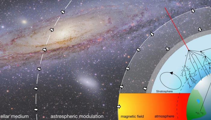
Thanks to the invention of the Neutron Monitor in 1948 and multiple spacecraft which monitor the cosmic ray environment since 1970’s we now have a constant record of the solar activity over almost 70 years. Information prior to this space era, however, are rare and take us back in time only to the late 1930s, when ionization chambers have been introduced. This of course allows us only a narrow view on the solar behaviour compared to the age of the Sun and our solar system and big scientific questions concerning, e.g., the current solar cycle can not be answered as easily. However, because galactic cosmic rays interact with the surrounding atmospheric constituents once they enter the atmosphere they are also able to induce the production of so-called cosmogenic radionuclides such as 10Be, 14C and 36Cl, with half-life times of up to 1.39 million years. Luckily, once mixed in the Stratosphere and Troposphere, these radionuclides get attached to aerosols and therewith transported to the surface. Here they are deposited in natural archives like ice sheets, tree rings or sediments, where the information of the solar activity is stored. Thus, cosmogenic radionuclides offer the unique possibility of obtaining a solar activity record over thousands of years. However, although cosmogenic radionuclide measurements can, thus, in principle be used to reconstruct solar activity back in time, in order to understand the underlying physical processes as detailed as possible the production of the cosmogenic radionuclides has to be studied numerically. As shown in Fig. 1, thereby a variety of complex physical processes has to be addressed, starting with the particle population of galactic cosmic rays in the local interstellar medium, their modulation within the heliosphere, their transport in the Earth’s magnetosphere as well as their interaction within the terrestrial atmosphere.
Prior to the end of 2012 the unmodulated galactic cosmic ray (GCR) flux, also known as the local interstellar spectrum (LIS), had not been measured in-situ. But with Voyager I crossing the outer heliosphere at around 122 AU for the first time measurements of the low energy LIS (below ~500 MeV) became available and the existing models on the production of cosmogenic radionuclides had to be revised.
Once GCR particles enter the heliosphere they encounter the heliospheric magnetic field (HMF) which is carried outwards by the solar wind. Thereby, the lower energy GCRs are modulated as they traverse the HMF. This transport can be described by the Parker transport equation, taking into account five important terms: the outward convection by the solar wind, gradient and curvature drifts in the global HMF, the diffusion through the irregular HMF, adiabatic energy changes due to the divergence of the expanding solar wind, as well as local sources (e.g., particles accelerated at the Sun). However, most often the much simpler analytical force-field approximation, which depends only on the solar modulation parameter Φ, is used in the literature. Furthermore, nowadays instruments like, e.g., PAMELA and AMS02 measure the high-energy GCR component above 10 GeV in the Earth’s vicinity, which is not influenced by the modulation due to the HMF. The energy spectrum of the energy range most important for the production of the cosmogenic radionuclides (0.4 – 8 GeV), however, is still unknown.
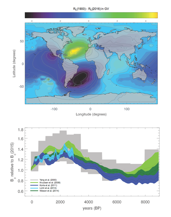
Figure 2: Upper panel: Annual variations computed with the IGRF model. Shown is the difference between the cutoff rigidities as they were present in 1900 and the ones of 2016. Lower panel: Comparison of the paleo-geomagnetic field reconstructions by different groups relative to present magnetic field strengths. Courtesy: K. Herbst
The HMF, however, is not the only magnetic filter that CRs encounter on their way to the Earth’s atmosphere. The Earth’s magnetic field also plays a major role when it comes to the modulation of the CR spectrum on top of the atmosphere. Although low- as well as high energy particles can enter the atmosphere at polar regions only high energy CRs can do so at equatorial regions. There is, however, not only a spatial but also temporal variation that has to be addressed. These changes can be of short term, e.g. due to a strong solar particle events, on the basis of annual variations (see upper panel of Fig. 2) but also centennial time scales (see lower panel of Fig. 2). Thus, such changes influence the primary particle spectrum on top of the atmosphere, and therewith the production of 10Be, 14C and 36Cl.
The main motor for the production of 10Be, 14C and 36Cl are galactic cosmic rays (GCRs) consisting of ∼87% protons, ∼12% alpha particles and ∼1% heavier particles (see e.g. Simpson, 2000). Once inside the Earth’s atmosphere CR induce the evolution secondary particle cascades of muonic, electromagnetic as well as hadronic origin. In particular the high energy secondaries of the latter are able to further interact with the atmospheric Nitrogen, Oxygen and Argon atoms due to spallation reactions as well as thermal neutron capture producing the terrestrial 10Be, 14C and 36Cl isotopes. Thus, there is a clear anti-correlation to the solar activity. As a consequence, during high solar activity the production of cosmogenic radionuclides is low, and vice versa.
After stratospheric- and tropospheric mixing on time-scales in the order of around two (10Be) up to twelve years (14C) cosmogenic radionuclides are being attached to aerosols and finally deposited in natural archives like ice sheets, tree rings or sediments, where the information of the solar activity of thousands of years is stored. Existing radionuclide records thereby showed that GCRs most likely are not the only CRs contributing to the production of cosmogenic radionuclides. Recently, unexpected production rate increases around 774/5 AD and 993/4 AD in all three records were observed. This started a fruitful scientific debate about the causes of such strong increases. With a multi-radionuclide approach of highly resolved 10Be records combined with 36Cl ice core data, in 2015 different scientific groups independently could infer that enormous solar eruptions were the most likely causes behind the observations.
By combining numerical modelling and observations it is possible to reconstruct the solar activity (in form of the solar modulation parameter Φ) back in time. A reconstruction based on 10Be records by Muscheler et al. (2007) is shown in Fig. 3. Amongst others, thereby the reconstruction strongly depends on the LIS model the numerical simulations are based on.
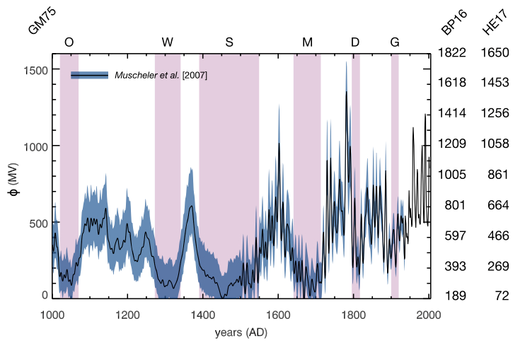
Figure 3: Reconstruction of the solar modulation parameter from 10Be measurements based on Muscheler et al. (2007). Courtesy K. Herbst
Nevertheless, one feature can be seen in all records: the so-called Grand Solar Minima, in which the Sun showed unusually long solar minimum activity over tens of years. Shown here are the reconstructions between AD1000 and AD2005, where six of these minima have occured: Gleisberg (1880-1914), Dalton (1790-1820), Maunder (1645-1715), Spörer (1450-1550), Wolf (1280-1350) and Oort (1040-1080). This immediately implies that the low solar activity observed in the current solar activity cycle is not that uncommon, and that we are well within another small Grand Solar Minimum (referred to as Eddy Minimum).
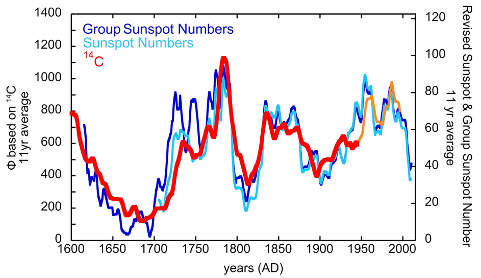
Figure 4: Comparison of the 14C – based solar-modulation parameter with the revised sunspot (light blue) and group sunspot (blue) numbers. All records show an running 11-year average. The red curve shows the 4C (neutron monitor)-based results of the numerical production calculations. Courtesy K. Herbst
In order to test the results a comparison of the reconstructed solar modulation parameter values with the sunspot number, which is a direct measure of the solar activity, can be performed. As can be seen in Fig. 4, a reasonably good agreement can be found. Furthermore, because the solar modulation parameter mathematically can also be linked to the HMF it is also possible to reconstruct the heliospheric magnetic field strength back in time and compare actual observations with geomagnetic-, sunspot number- as well as 10Be-/14C- based reconstructions. As can be seen in Fig. 5 an impressive correlation between the different records has been found.
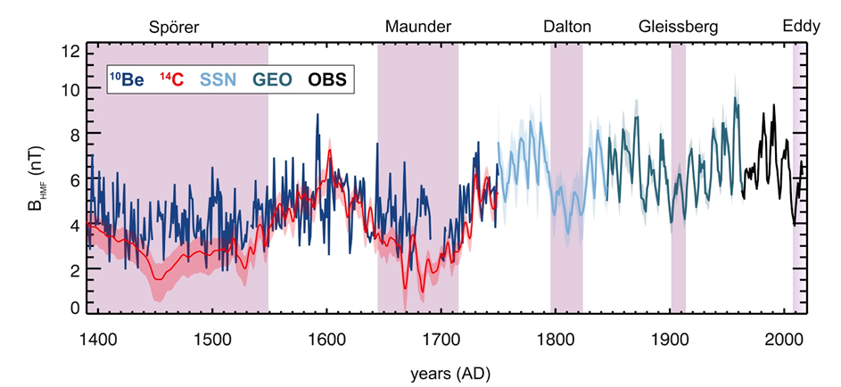
Figure 5: Composite plot of the reconstructed heliospheric magnetic field strength from 1390–2016 based on cosmogenic 10Be (McCracken and Beer 2015; 1391–1748), 14C (Muscheler et al. 2016; 1390–1748), the sunspot number (Owens et al. 2016a; 1749–1844), geomagnetic data (Owens et al. 2016a; 1845–1964), and from near-Earth observations in space (1965–2016). Courtesy K. Herbst
For more background information the reader is referred to the publications by:
Beer, McCracken and von Steiger, Springer Business & Media (2012), https://doi.org/10.1007/978-3-642-14651-0
Muscheler et al. (2016), Solar Phys., https://doi.org/10.1007/s11207-016-0969-z
Cliver and Herbst (2018), Space Sci Rev, 214:56, https://doi.org/10.1007/s11214-018-0487-4
This post was writtend by Dr Konstantin Herbst

Dr Konstantin Herbst from the Christian-Albrechts-Universität zu Kiel, Germany