the Creative Commons Attribution 4.0 License.
the Creative Commons Attribution 4.0 License.
 | 10 Jul 2019
Atmospheric measurements of the terrestrial O2 : CO2 exchange ratio of a midlatitude forest
Mark O. Battle
J. William Munger
Margaret Conley
Eric Sofen
Rebecca Perry
Ryan Hart
Zane Davis
Jacob Scheckman
Jayme Woogerd
Karina Graeter
Samuel Seekins
Sasha David
John Carpenter
Measurements of atmospheric O2 have been used to quantify large-scale fluxes of carbon between the oceans, atmosphere and land since 1992 (Keeling and Shertz, 1992). With time, datasets have grown and estimates of fluxes have become more precise, but a key uncertainty in these calculations is the exchange ratio of O2 and CO2 associated with the net land carbon sink (αB). We present measurements of atmospheric O2 and CO2 collected over a 6-year period from a mixed deciduous forest in central Massachusetts, USA (42.537∘ N, 72.171∘ W). Using a differential fuel-cell-based instrument for O2 and a nondispersive infrared analyzer for CO2, we analyzed airstreams collected within and ∼5 m above the forest canopy. Averaged over the entire period of record, we find these two species covary with a slope of mol of O2 per mole of CO2 (the mean and standard error of 6 h periods). If we limit the data to values collected on summer days within the canopy, the slope is . These are the conditions in which biotic influences are most likely to dominate. This result is significantly different from the value of −1.1 widely used in O2-based calculations of the global carbon budget, suggesting the need for a deeper understanding of the exchange ratios of the various fluxes and pools comprising the net sink.


Since the pioneering work of Keeling and Shertz (1992), measurements of the abundance of atmospheric O2 and CO2 have been used extensively for constraining fluxes of carbon to and from the land biosphere and the oceans. In a conceptual form, the budgets for atmospheric O2 and CO2 can be written
where fxx is the flux of CO2 from reservoir xx to the atmosphere, αff is the global average oxidative ratio of fossil fuels, and αB is the average oxidative ratio of the global net land carbon sink. Zocean describes the outgassing of O2 from the ocean due to warming. Knowing fff and αff from industrial inventories, calculating Zocean from changes in ocean heat storage, and measuring the changes in O2 and CO2, we can solve these two equations for fland and focean in terms of αB (for a rigorous treatment of these equations, see for example Keeling and Manning, 2014). This O2-based method has become increasingly sophisticated with refinements in methodology, and increasingly precise with better instruments and ever-longer datasets (Keeling and Manning, 2014). Nonetheless, all estimates of global carbon fluxes based on atmospheric O2 require a value for αB.
The molar ratio of O2 released to the atmosphere and CO2 removed from it during photosynthesis (one contribution to αB) will depend on the type of organic material being synthesized. This ratio is set by the relative amounts of carbon and hydrogen in the material, as well as the amount and source of any nitrogen included. Similarly, the ratio of CO2 release and O2 uptake during respiration depends on the composition of the material being respired and whether nitrogen is oxidized to nitrate. For example, synthesis and respiration of the simplest sugar (glucose: C6H12O6) will have a flux ratio of 1.0. However, if plants are making shoots and other nitrogen-rich tissue, the oxidative ratio might range from 1.0 to 1.26, depending on the source of the nitrogen (nitrate vs. ammonium) (Bloom et al., 1989). Clearly, any value of αB that is used in a large-scale calculation of carbon fluxes must represent the net imbalance of many processes in many ecosystems over long times.
One approach to this problem is to survey the elemental ratios of various biogenic materials. This was done by Severinghaus (1995), Randerson et al. (2006), Masiello et al. (2008), Hockaday et al. (2009), Worrall et al. (2013), and Gallagher et al. (2017). Based on a variety of techniques and a range of materials, estimates of αB at present seem to be around 1.05±0.1 (Keeling and Manning, 2014). Propagating this uncertainty to the global land–ocean partition of carbon uptake yields a value of ±0.1 PgC yr−1.
One method that can illuminate the processes responsible for αB, and the one we have chosen, was first published by Seibt et al. (2004), Sturm et al. (2005), and Stephens et al. (2007). It uses direct measurements of O2 and CO2 changes in ambient air within, and close to, an ecosystem. Given sufficient precision and temporal resolution, the covariation in these two atmospheric components should reflect the exchange ratio for the particular mixture of fluxes to/from the ecosystem present during the study period. We refer to this quantity as the local biotic exchange ratio (LBER), recognizing that it is closely related to, yet distinct from, αB. αB may turn out to be close to measured values of LBER, but it is a distinct quantity by definition: αB is the ratio of global net CO2 and O2 exchanges from all terrestrial biological processes.
The most groundbreaking feature of the work of Stephens et al. (2007) was the use of a newly developed, continuous O2 analyzer deployed at the study site, allowing precise, high-frequency measurements. These techniques have the potential to better characterize contributions to αB as well as improve our understanding of the underlying physiology of the ecosystem generating the fluxes.
Following Stephens et al. (2007), we have used a fuel-cell-based differential O2 analyzer and a nondispersive infrared (NDIR) CO2 analyzer to make quasi-continuous measurements of the air in and above the canopy at the Harvard Forest Environmental Measurement Site (Urbanski et al., 2007). In the following sections of this paper, we begin with a description of the instrument and our methods of data collection and analysis. We then present data acquired between 2006 and 2013 and make a first effort at interpreting these data in the context of both the ecosystem's process-specific ratios and the response of the ecosystem to environmental controls.
A note on units: because O2 is a major atmospheric constituent, its abundance is customarily reported in per meg defined as
where O2∕N2st is O2∕N2 for the standard gas on which the scale is based. This avoids complications arising from dilution effects (Keeling et al., 1998). Because our measurements are made using an instrument that reports differences in apparent mole fraction, we convert to per meg using Eq. (3) of Stephens et al. (2007). Finally, when working with exchange ratios, we convert per meg to parts per million equivalent by multiplying per meg by 0.209500 (the O2 mole fraction of atmospheric air) (Keeling et al., 1998). When using parts per million equivalent for O2 and micromole per mole (or parts per million) for CO2, the synthesis of glucose (described above) would increase O2 and decrease CO2 by an equal number of units, directly translating our measurements to the underlying stoichiometry, as desired.
In August 2005 we installed a measurement system at the Harvard Forest Environmental Measurement Site (EMS). Located at 42.5377∘ N, 72.1714∘ W and 340 m above sea level, we collected air from two intake tubes mounted on a tower 7.50 and 29.0 m above the ground. The lower intake is within the forest canopy, the upper about 5 m above it. The tower and site are described in more detail by Urbanski et al. (2007). Our system is very similar to the one installed at WLEF radio station in Wisconsin and documented very thoroughly by Stephens et al. (2007), so we focus primarily on differences from the WLEF instrument in our description here.
2.1 System design and operation
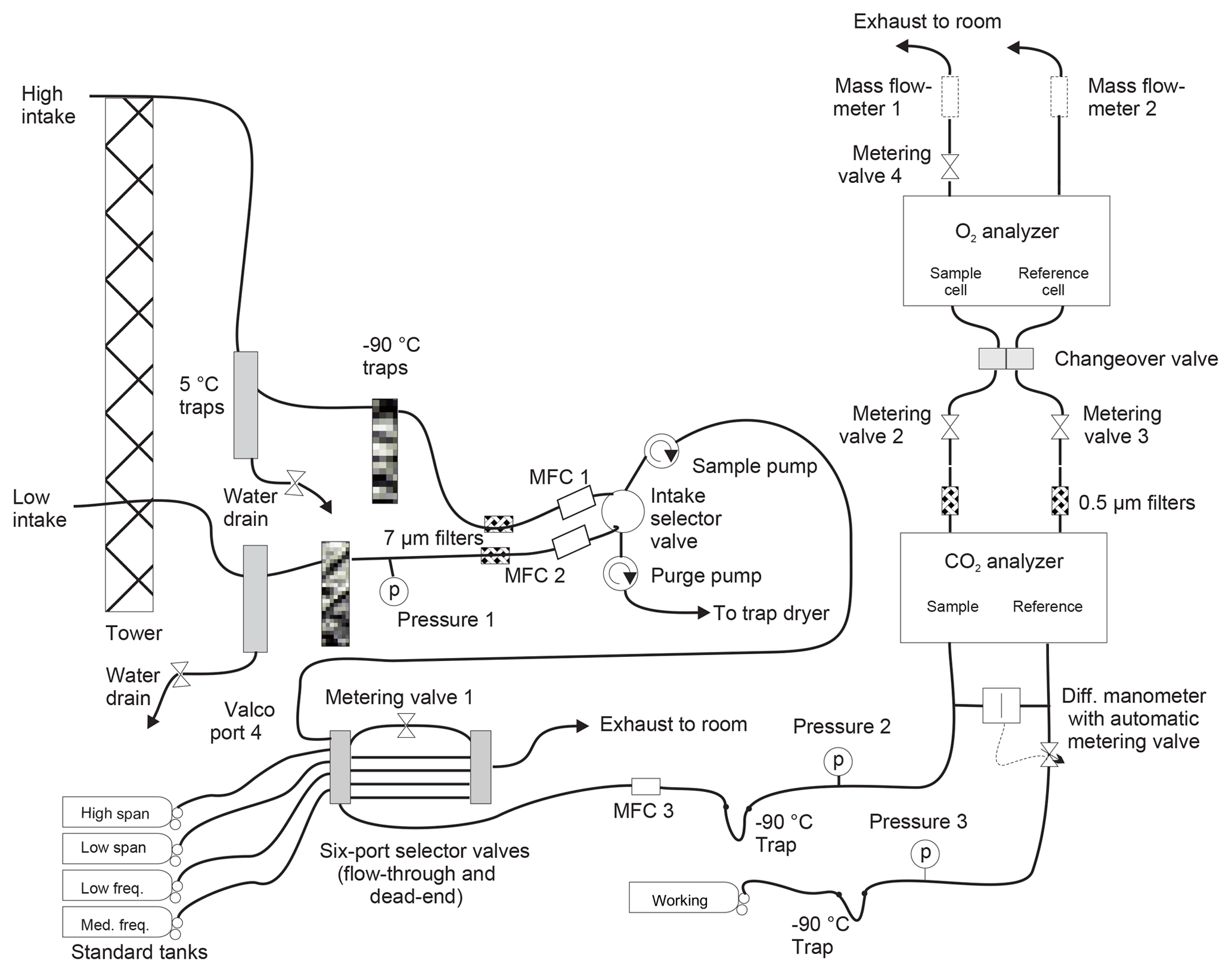
A schematic of the system is shown in Fig. 1. Unless otherwise mentioned, all wetted surfaces are stainless steel. At both points of collection, air is drawn in through downward-facing aspirated inlets (R.M. Young, part no. 43408) to reduce thermal fractionation (Blaine et al., 2006). A nominal flow rate of 50 cm3 min−1 is maintained at all times in both lines using pumps with Viton diaphragms and PTFE valves (KNF Neuberger N05-ATI) in concert with mass flow controllers (MKS M100B). Tubing on the tower ( Dekabon®) is routed into the instrument enclosure without local low spots to minimize buildup of condensed water. Within the building, water is removed from the airstream using a series of three coaxial stainless steel traps. The first is kept at 5 ∘C with a Peltier cooler (M&C model ECP2000-SS), while the second and third traps are filled with borosilicate glass beads and immersed in a heat-transfer fluid (Syltherm XLT®) held at −90 ∘C using a mechanical refrigeration system (FTS VT490). Filters with a nominal pore size of 7 µm (Swagelok SS-6F-7) protect downstream equipment from particulates. Since our analyzers can only measure a single airstream, the high and low intake lines are alternately sent to analysis or waste. The intake selector valve is a pneumatically actuated, crossover ball valve with PTFE packing (Swagelok SS-43YFS2), switched every 720 s.
Both the O2 and CO2 analyzers make differential measurements of the chosen stream of ambient air relative to a cylinder of dried air (the working tank, WT). Data are recorded at 1 Hz. Periodically, the ambient air stream is diverted to waste and the WT is analyzed against one of four calibration tanks: HS, LS, MF, and LF. Details of the various tanks are given in Table 1. The frequency of the calibration runs was determined in part from pre-deployment tests in which we observed instrumental drift when running pairs of (sacrificial) tanks against one another. Other considerations include consumption of standard gases and lost time for atmospheric measurements.
Table 1Nominal composition of calibration tanks. Actual values vary slightly as cylinders are used and refilled. The O2 values quoted here were measured in the lab of R. Keeling, while the CO2 values were measured by the CCGG lab of NOAA ESRL GMD. Based on replicate measurements, the O2 values are typically determined to within roughly ±1.5 per meg on the S2 scale, while the CO2 values on the WMO X2007 scale are known to about ±0.2 µmol mol−1 (Hall, 2017). The cylinders are Luxfer N265 uncoated aluminum, with 51-14B regulators from Scott Specialty Gases (now Air Liquide). Tanks and regulators are stored horizontally in an insulated box to minimize thermal and gravitational fractionation.

The ambient air stream (high or low) or the calibration tank is chosen for analysis with a pair of electrically actuated six-port selector valves (VICI EMT2SF6MWE and EMT2SDMWE). From these valves it passes through another mass flow controller, the NDIR CO2 analyzer (Li-cor LI-7000), a 0.5 µm filter (Swagelok SS-6F-05), a needle-tipped metering valve (Swagelok SS-4BMG), a changeover valve assembly (four Numatics TM101V24C2 solenoid valves on a custom-built aluminum manifold), and the fuel-cell-based O2 analyzer (Sable Systems Oxzilla II with customized stainless steel internal plumbing), and then exits through a mass flowmeter (Honeywell AWM3100V). Absolute pressures are recorded upstream of the CO2 analyzer in three locations (Omega PX303-030A10V) and within the Oxzilla instrument (see below).
The response of the Li-cor CO2 analyzer depends on the pressure difference between the two cells. Thus, we use a differential manometer and electronically controlled metering valve with active feedback (MKS 223BD, 247D, and 248) to ensure balanced pressures in the Li-cor analyzer.
The response of the Oxzilla O2 analyzer depends on both pressure and flow differences between the cells. To provide sufficient control of these parameters, we have two metering valves upstream of the Oxzilla and one downstream. We use the metering valves (as well as the active pressure-difference control upstream of the Li-cor) to tune the system so that pressures and flows are as close to equal as possible regardless of the state of the changeover valve (see below). For this tuning, and subsequent monitoring of the system, we use flow data from the Honeywell meters and pressure data recorded within the Oxzilla immediately downstream of the cells. Prior to deployment, we modified the Oxzilla's internal plumbing and electronics so that pressure transducers (Honeywell SCX15N) were teed off of each of the outlets of the fuel cells. The two transducers are read out with the single high-precision digitizer built into the Oxzilla motherboard using a multiplexer to alternately select the transducer signal sent to the digitizer.
To further improve measurement precision of O2, we follow Stephens et al. (2007) and use a changeover valve to alternate the fuel cells into which the two gas streams flow. This allows for a difference-of-difference calculation that eliminates cell-to-cell biases in the instrument. However, the elimination of bias occurs only if that bias varies little during the two measurement periods being considered. Achieving optimal precision would seem to require high-frequency changeovers to reduce variation in the bias. However, each changeover is followed by a “dead time” when flows and instrument response need to settle. For a given dead time, more rapid changeovers mean fewer measurements are available for averaging, leading to a greater impact of random noise and thus poorer precision.
We adopt a method for quantifying this trade-off and settling on an optimal changeover frequency that was developed by Keeling et al. (2004). We determined dead time for our instrument by analyzing tank air (relative to a working tank) with the changeover running very slowly. We then measured the time after each changeover required for O2 values to settle to within 1σ of the post-changeover equilibrium value. This dead time was 14 s for our instrument. We then determined the optimal changeover time by analyzing two tanks of air against each other with the changeover valve disabled. We processed these measurements as if the changeover valve were operating, calculating difference-of-difference values for various (hypothetical) changeover rates, imposing a 14 s dead time. This exercise indicated an optimal changeover rate of 24 s between switches.
2.2 Data reduction
2.2.1 Atmospheric data
In order to allow the instrument to achieve equilibrium after the selector valves have changed state (at the end of a calibration run), we discard the first 432 s of atmospheric data after such an actuation.
The remaining atmospheric data are naturally divided into 12 min subsets by the switching of the intake selector between high and low intake lines. We discard the first 432 s of data after an intake switch to allow time for the instrument to re-equilibrate after the disruption in flows and pressures. The surviving data are processed slightly differently for O2 and CO2.
For O2, we break the surviving 288 s of data into 24 s blocks defined by the cycling of the changeover valve. We average the 1 Hz data collected between 14 and 24 s after the valve changes state. We then calculate difference-of-difference values for consecutive pairs of averages. This typically yields six values. These are in turn averaged, yielding a single O2 value for the chosen intake height at a time corresponding to the middle of the interval of data used in the average.
For CO2, we consider every 1 Hz CO2 value collected at the same time as the 1 Hz O2 values that contribute to the final O2 mixing ratio for each of the 12 min intake intervals. After the cuts for dead time following valve actuation (gas selector, intake selector, and changeover), there is 120 s of live data, so our CO2 mixing ratio is an average of 120 measurements.
2.2.2 Calibration data
Roughly four times daily, atmospheric sampling is interrupted for 6 min runs of calibration tanks. To more effectively use the information from these runs, we adopt a protocol that differs from our treatment of atmospheric data.
To flush stale gas from the lines and purge the regulators, air from the calibration tank is vented to waste for 6 min prior to measurement. Once the selector valves direct the calibration air to the analyzers, we consider all 6 min of CO2 measurements. We look for a transition in the CO2 value as tank air reaches the analyzer, displacing the atmospheric air that was in the optical cell. We find the time at which 70 % of the eventual change in CO2 has been achieved (the transition time).
To determine O2 in these calibration runs, we calculate difference-of-difference values for each pair of changeover blocks as with our atmospheric data. Then, based on the timing of the transition in the CO2 record, we average the last three, four, or five difference-of-difference values of the calibration run. The transition time typically occurs ∼2.6 min after moving the selector valve. In this case, we average three difference-of-difference pairs, corresponding to the last 2.4 min of data. This translates to averaging the last ∼40 % of each calibration run (or ∼70 % of the post-transition data).
To determine CO2, we average all CO2 values collected at the same times as the values that were used in the O2 calculation.
Our standards are calibrated on the Scripps S2 O2 scale (Keeling et al., 1998, 2007) and the NOAA/WMO CO2 scale (Zhao and Tans, 2006), thanks to the generous assistance of these laboratories. Thus it is on these scales that we report our measurements.
2.3 System performance
While we have made great efforts to calibrate our measurements to internationally accepted CO2 and O2 scales using our suite of reference tanks (Table 1), we defer a detailed treatment of long-term measurement stability and accuracy for a later publication. Our focus in this paper is on the local biotic exchange ratio, as expressed in a series of short-term averages of CO2 and O2 covariation. Thus, our primary concern is instrumental precision and stability over periods of roughly 6 h.
To determine this instrumental precision, we use runs of calibration tanks (see Sect. 2.2.2).
There are two possible approaches: we could use the observed scatter in the three, four, or five difference-of-difference values for O2 that are calculated during a 6 min run of a calibration tank, and likewise for the 60, 80, or 100 CO2 measurements retained during the same run. These are the values plotted in Fig. 2. We refer to this metric as “scatter on one tank” (SOOT).
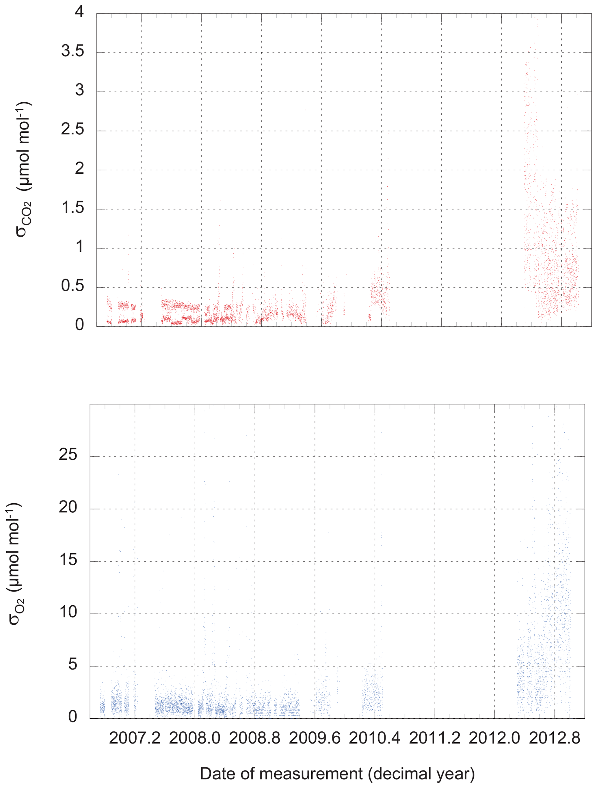
Figure 2The scatter (standard deviation from the mean) of routine CO2 and O2 measurements of calibration tanks. Values plotted here apply to individual CO2 measurements (1 Hz) and single difference-of-difference O2 values (one value every 48 s).
Not surprisingly, the performance of the instrument varies over time. At times, we could link a loss of precision to problems with an individual analyzer, while on other occasions, we found water (liquid or solid) in the system to be the cause. The source of the major degradation in the precision of both analyzers that develops in late 2012 and persists until the end of our dataset remains under investigation.
An alternative approach, and the one that we adopt here, uses the observed scatter in the difference of paired standard tanks that were run immediately following one another. The calculation of the difference between the HS and LS tanks run in succession emulates the treatment of the atmospheric data by comparing one gas stream (HS in place of atmosphere) to another (LS in place of a “calibration curve”) without the involvement of the working tank. The scatter in the HS–LS difference is a conservative estimate of uncertainty in atmospheric data because it includes any variability that might be introduced by operation of the gas-selection valve, a valve that remains fixed in position during atmospheric sampling.
We find the scatter in the HS–LS differences for 12 d periods is around ±2 ppm equivalent for O2 and ±0.2 µmol mol−1 for CO2 until the middle of 2008. From 2012 onward, the scatter was ±9 ppm equivalent and ±0.6 µmol mol−1.
Each HS and LS O2 value was typically the average from three difference-of-difference pairs, while the CO2 values were usually an average of 60 measurements. In contrast, a 12 min atmospheric measurement on either the high or low intake is an average of six O2 difference-of-difference pairs and 120 CO2 measurements (Sect. 2.2.1). Thus, the atmospheric measurements should have uncertainties given by
Based on these equations, we believe that the atmospheric measurements carry uncertainties of ppm equivalent and µmol mol−1 prior to mid-2010. For measurements beginning in 2012, the uncertainties were ppm equivalent and µmol mol−1.
Our choice to work backwards from the observed scatter in HS–LS pairs may not be the optimal technique for extracting uncertainties, but we are confident it yields O2 and CO2 errors that bear the correct relative size. Thus, we use the value listed above when calculating slopes in our Deming regressions (Sect. 3).
The measurements we present here commenced on 27 September 2006 and continued until 9 January 2013. The record is approximately continuous until the middle of 2010, when a series of hardware failures, due in part to a lightning strike, caused an extended hiatus in data collection. Measurements resumed in May 2012 and continued without interruption through the end of that year, when failure of the oxygen analyzer led to a suspension of data collection.
Measurements of O2 and CO2 for the entire period of record are shown in Fig. 3, while Fig. 4 gives an example of a single day's cycle. The values shown here were derived from the raw data using the calibration runs and the algorithm described in Sect. 2.2. They represent our best estimates of the O2 and CO2 content of the atmosphere on the Scripps S2 and NOAA–WMO scales, respectively. In these figures we can see a very gradual rise in CO2 and drop in O2 (mainly due to fossil fuel combustion), a strong diel cycle with inverse variation in CO2 and O2, and a great deal of variability on a range of timescales. Results from the upper and lower intakes are quite similar, but not identical.
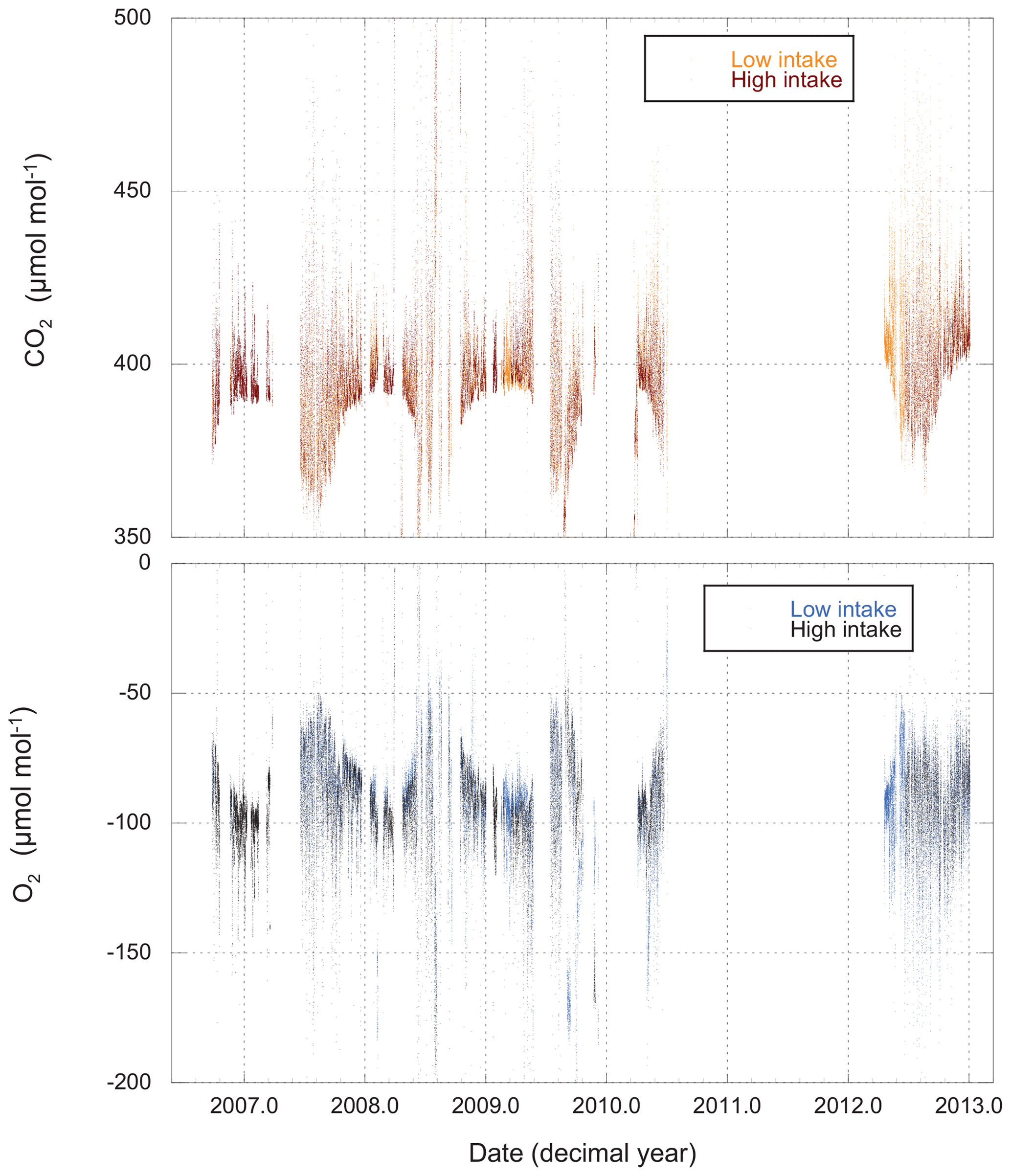
Figure 3CO2 and O2 measured from both high and low intakes at Harvard Forest. The data have been processed (Sect. 2.2) and are presented on the WMO and S2 scales. Each point (spaced 11 min apart) represents the average atmospheric composition for a 4.8 min period.

Figure 4A detailed look at Fig. 3. CO2 and O2 measured from the high intake on 29 September 2006. This is simply one example of the diel cycle of these species. Note the strict inverse variation in O2 and CO2, even when there are large deviations from a smooth temporal evolution.
While these records contain a wealth of information, our particular focus is on the covariation in O2 and CO2. We expect to see different results from the high and low intakes, particularly at night. The lower intake is more likely to show stronger influences of soil and canopy fluxes, particularly at night when the atmosphere is more stable and the surface layer is more likely to be decoupled from the planetary boundary layer. For this reason, we separate the data from the high and low intakes, create day and night subsets for each intake, plot O2 vs. CO2 for each subset, perform a linear regression, and take LBER from the slope of the fit.
The 6 h subsets making up each plot are 09:00–15:00 LT (day) and 22:00–04:00 LT (night). These intervals are chosen to be times of maximal and minimal coupling (day and night, respectively) between the air within and above the canopy. We define the intervals based on the climatological diel cycle in the friction velocity u* measured at the EMS tower (Munger and Wofsy, 2017). Subsets with fewer than three measurements are ignored. Because uncertainties in both species are comparable, we use a Deming regression (Deming, 2011). Furthermore, to reduce any influence of non-Gaussian tails in the dataset, we perform an iterative fit, in which we calculate the standard deviation of the residuals to the fit (σres) and discard any points lying more than 4σres from the fit. Of the 3760 fits, only 50 had any outliers and only 11 of these required more than one iteration to converge. Representative plots and fits are shown in Fig. 5.
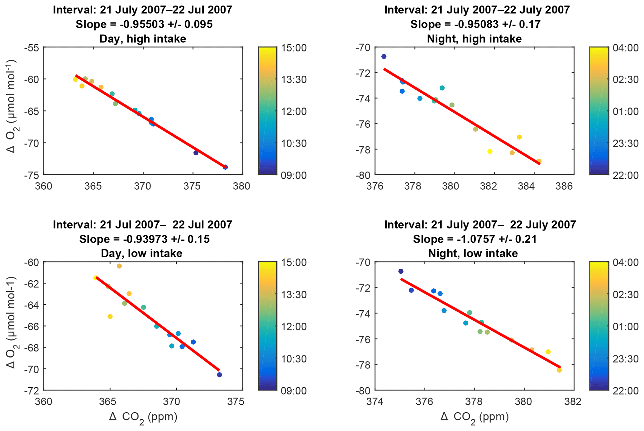
Figure 5Representative examples of slope plots: data collected during day and night periods from the high and low intakes on 21–22 July 2007. The colors of the points indicate the time of collection within the 6 h intervals, as keyed in the color bar to the right of each plot. Errors on the slopes are purely statistical.
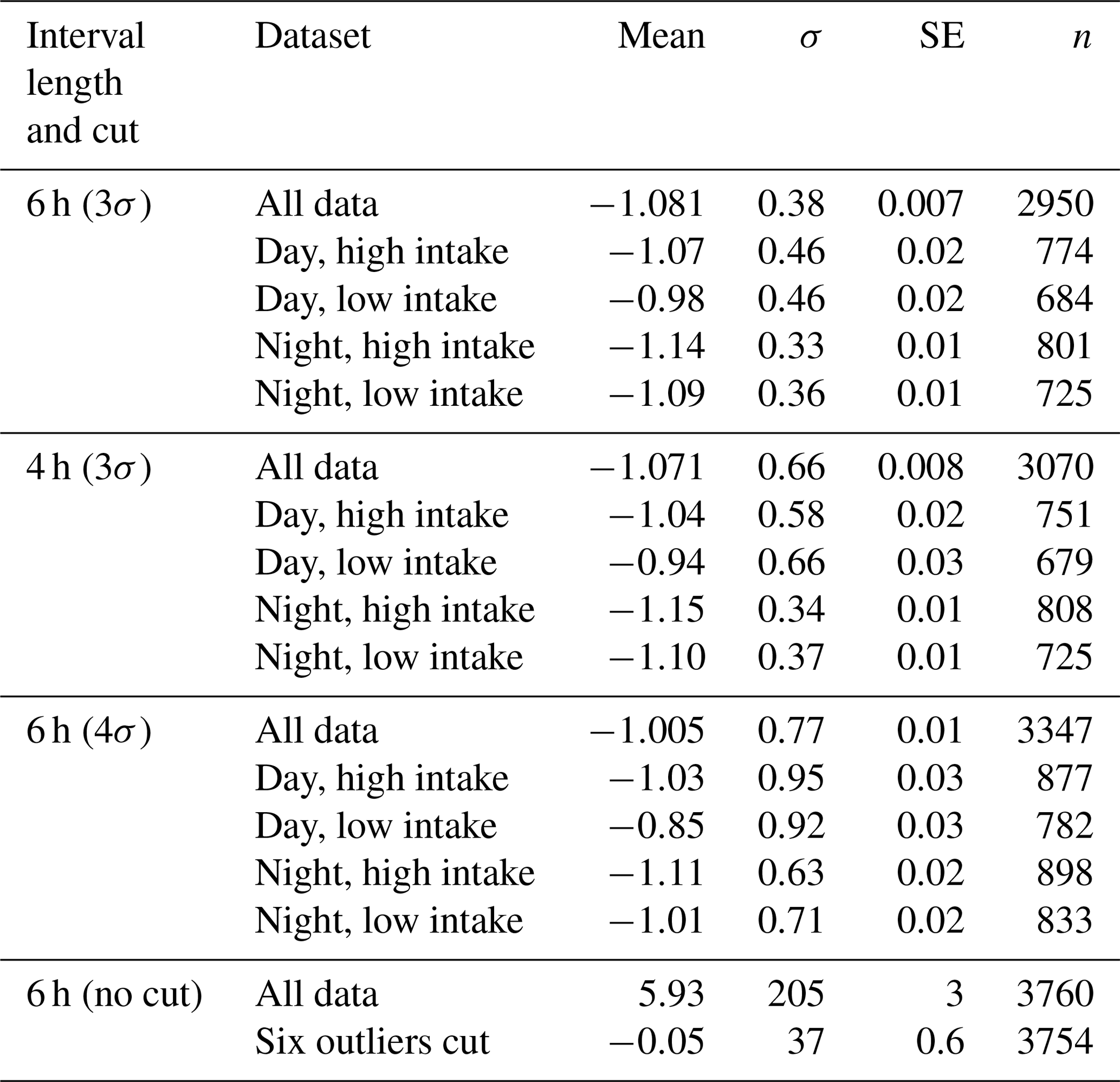
In total, we have slope values for 3760 6 h subsets. While the great majority of slope values are close to −1.0 and are normally distributed (see Fig. 6), a small number are implausibly large (up to +2035.9) or small (down to −102.6). Since we seek a representative slope value for each high–low day–night subset, we choose to limit the impact of these outliers by performing an iterative calculation of the means. We calculate a mean and standard deviation, discard all slopes more than 3σ from the mean, and iterate to convergence. Table 2 shows the results of these calculations, as well as sensitivity studies varying the length of the day and night intervals and the tightness of the cut in our iterative averaging.

Figure 6Probability plots of slopes for the entire dataset, before and after a 3σ iterative cut. The dashed–dotted lines indicate the shape expected for a purely Gaussian distribution. In the interests of clarity, we omit five points with extremely large or small slopes from (a). See Table 2 for statistical details of these distributions.
Table 2Table of average values for all slopes and four data subsets. σ is 1 standard deviation, SE is the standard error of the mean (), and n is the number of slope values surviving the iterative cut.
In its simplest form, the variability in O2 and CO2 in the continental interior is an end-member mixing problem: fossil fuel fluxes will give slopes ranging from −1.17 (coal) to −2.0 (methane) (Keeling, 1988; Steinbach et al., 2011), while biogenic fluxes will give slopes closer to −1.0. Thus, we expect air masses exposed to both types of fluxes will evolve with intermediate slopes.
Within this conceptual framework, a successful effort to extract LBER from the data depends on the relative sizes of the biogenic and anthropogenic fluxes. Only at times when photosynthesis and respiration dominate the land–air fluxes will observed slopes be close to LBER.
To test these assertions, we first use a Lagrangian transport model to estimate the region over which surface fluxes influence signals at our sampling site. We then use a simple one-dimensional box model to establish the validity of the end-member mixing framework. Finally, we estimate the relative size of the biogenic and anthropogenic contributions.
4.1 The 6 h provenance of atmospheric variability
We use a Lagrangian transport model to estimate the surface regions to which air parcels are exposed during the 6 h prior to their arrival at the EMS tower. Specifically, we created back-trajectories for a range of dates and times, day and night, across seasons and years using the HYSPLIT Lagrangian transport model (NOAA, 2018) forced with NAM12 meteorology. We generated many sets of six 6 h back-trajectories originating hourly during the daytime or nighttime intervals to determine the provenance of the air we analyze at Harvard Forest. An example of one such set of trajectories is shown in Fig. 7.
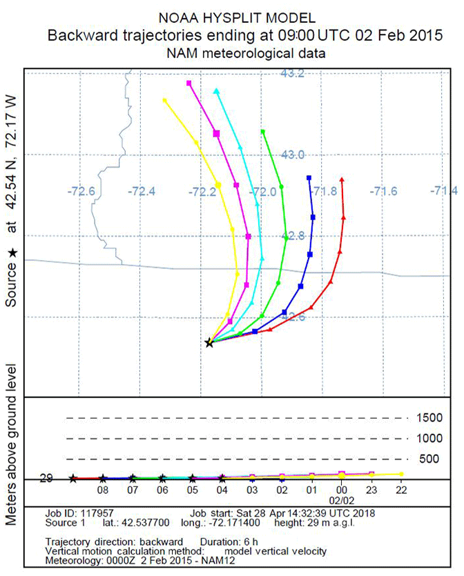
Figure 7An example of 6 h back-trajectories for Harvard Forest on 2 February 2015. Trajectories start hourly between 22:00 and 04:00 EST, corresponding to the nighttime interval for slope plots. State lines for New Hampshire, Vermont, and Massachusetts are in gray. On this particular night, the source region was fairly constant, so changes in O2 and CO2 are relatively likely to be primarily due to local influences.
In general, the 6 h provenance ranges from 50 to 200 km, with little spatial variation over the 6 h interval. Given the location of our study site, a ∼100 km provenance, primarily from the west, means the air we analyze has traveled over a mostly forested landscape, occasionally passing small urban centers. This analysis is consistent with the work of Gerbig et al. (2006), who found a 10-fold (or greater) falloff in the influence of fluxes more than ∼100 km from the study site.
4.2 “Mixing” of slopes
To test the applicability of an end-member approach, we considered the simplest model with two contributors: generic fossil fuel, with an exchange ratio of −1.4, and biotic activity, with an exchange ratio of −1.05. These characterized the stoichiometry of surface fluxes used in a one-dimensional box model, in which parcels of air travel forward in time in 12 min steps, passing over a fictitious landscape with forested, suburban, and urban components. In 30 of these time steps the parcels exchange CO2 and O2 with the underlying sources and sinks, changing the composition of the parcel according to
where C is the mixing ratio of O2 or CO2 in micromoles per mole, F is the flux from the landscape underneath the box in micromoles per square meter per second, t is the time step in seconds, h is the height of the box in meters, and the factors of 22.4 (the molar volume) and 1000 convert moles to liters and liters to cubic meters, respectively. For h we use one-half of the planetary boundary layer (PBL) height. We spin up the model for 24 h and then record O2 and CO2 concentrations of consecutive parcels as they “arrive” in their final time steps over the same 6 h day and night intervals used for the observations.
The CO2 surface fluxes vary with time of day and day of year and are based on observations at Harvard Forest (Munger and Wofsy, 2017) and in urban (Bergeron and Strachan, 2011; Velasco and Roth, 2010; Ward et al., 2015) and suburban (Bergeron and Strachan, 2011) settings. The O2 surface fluxes were derived from the CO2 fluxes by assuming exchange ratios of 1.4 for fossil fuel combustion and 1.05 for biospheric activity. The PBL values are climatological hourly average values, calculated separately for summer and winter from the NAM12 dataset (NOAA, 2018). Within the STILT model (Gerbig et al., 2006), only air within the lower half of the PBL is influenced directly by surface fluxes. Air above this height is closely matched to the composition of the free troposphere. Because we use the STILT model to infer the provenance of air we analyze, we define our box height as half the height of the PBL so that the two models (STILT and our 1-D box model) are conceptually consistent. We performed sensitivity studies, varying the landscape composition (ranging from 100 % forest to 100 % urban), surface flux magnitude (values characteristic of winter and summer seasons), and PBL height (25 %–75 % of the NAM12 values). In all cases, the CO2 and O2 values of the parcels entering the model were held constant, ensuring that any variability predicted by the model was a result of the fluxes from the landscape over which the parcels traveled in the previous 6 h and/or changes in PBL height.
We emphasize that the purpose of the 1-D model is to explore the validity of the end-member mixing approach. In particular, we ask whether a mix of sources will relate simply to a mix of slopes, despite the fluxes and the box height having their own diel cycles.
In all but a few special circumstances, the model predicts slopes that are completely consistent with the specified admixture of the source fluxes over which the air parcels have traveled. Exceptions arise when the covariation in the boundary layer height and diel cycles in the fluxes conspire to bias slopes by a few percent. Results of various sensitivity tests and a discussion of these exceptions can be found in Table 5.1 of Conley (2018), along with a more complete description of the model and its forcing fluxes.
The 1-D model results give us confidence that slopes close to −1.0 are a closer representation of the LBER, while more negative slopes have ever larger contributions from fossil fuel combustion. Though reassuring, we acknowledge the model results are not definitive due to the many simplifications involved. More sophisticated studies are needed to give a truly robust confirmation of the end-member mixing framework.
Aside from the slopes, the full range of O2 and CO2 variability predicted by the model is in the general range of our observations. Because of the crude nature of our model, this result is somewhat surprising. Our values for the box height and the molar volume are almost certainly wrong, so the data–model agreement may be coincidental.
Adopting the approach outlined above, we interpret slopes of our plots as averages of LBER (a number near −1.0) and external fossil fuel influences (numbers ranging from −1.17 to −2.0), weighted by the relative contributions of these fluxes in the Harvard Forest “footprint”.
Taking all data together, using 6 h intervals, we find a slope of (see Table 2). This value is a little higher than the oxidative ratio of organic material calculated by Worrall et al. (2013) and at the lower end of the range of possible values for the global exchange ratio quoted by Severinghaus (1995).
Ideally, our dataset would not include “poor” slopes – those that are weakly constrained by the data or unduly influenced by a small number of points. We found the most effective tool for excluding such slopes was a 3σ iterative cut. In practice, this cut only eliminates 6 h intervals with slopes that are positive, or very negative (). Inspection of a subset of the fits failing the cut shows they are indeed poor fits, as defined above. While the cut does not catch all poor slopes, we believe the slopes that are cut are poor ones.
We emphasize that this all-inclusive average slope is not a direct measurement of the LBER. Instead, it is a measure of the LBER mixed with the exchange ratio of fossil fuel combustion.
We also considered 2-week aggregation periods (instead of 6 h). These slopes average . This is consistent with nearly equal contributions from fossil and biotic fluxes, as expected for an aggregation period with a provenance encompassing the entire continental United States (Gerbig et al., 2006).
5.1 Information from subsets of data
Considering particular subsets of the data (Table 2) may provide insight into the processes determining observed slope values. Thus, we categorize our 6 h slopes by day and night, high and low, winter (December, January, February) and summer (June, July, August).
We begin with data aggregated in broad categories. Each group's average slope, calculated using the 3σ cut described above, is shown in Fig. 8. These groupings convey some unequivocal messages: summer slopes are less negative than winter slopes. Day slopes are less negative than night slopes. Low-intake slopes are less negative than high-intake slopes. Daytime data from the low intake are least negative of all.

Figure 8Average slopes for various subsets of the data. Error bars show the standard error on the mean. Subsets within each group (i.e., sharing a color) are nonoverlapping.
We also consider narrower categories, each with a unique set of slopes. The average slopes for each category are shown in Fig. 9. For these averages, we impose a 2.5σ iterative cut because a 3σ cut fails to reject several unphysical fits (with slopes >2.0) in the winter subsets, badly biasing the mean.
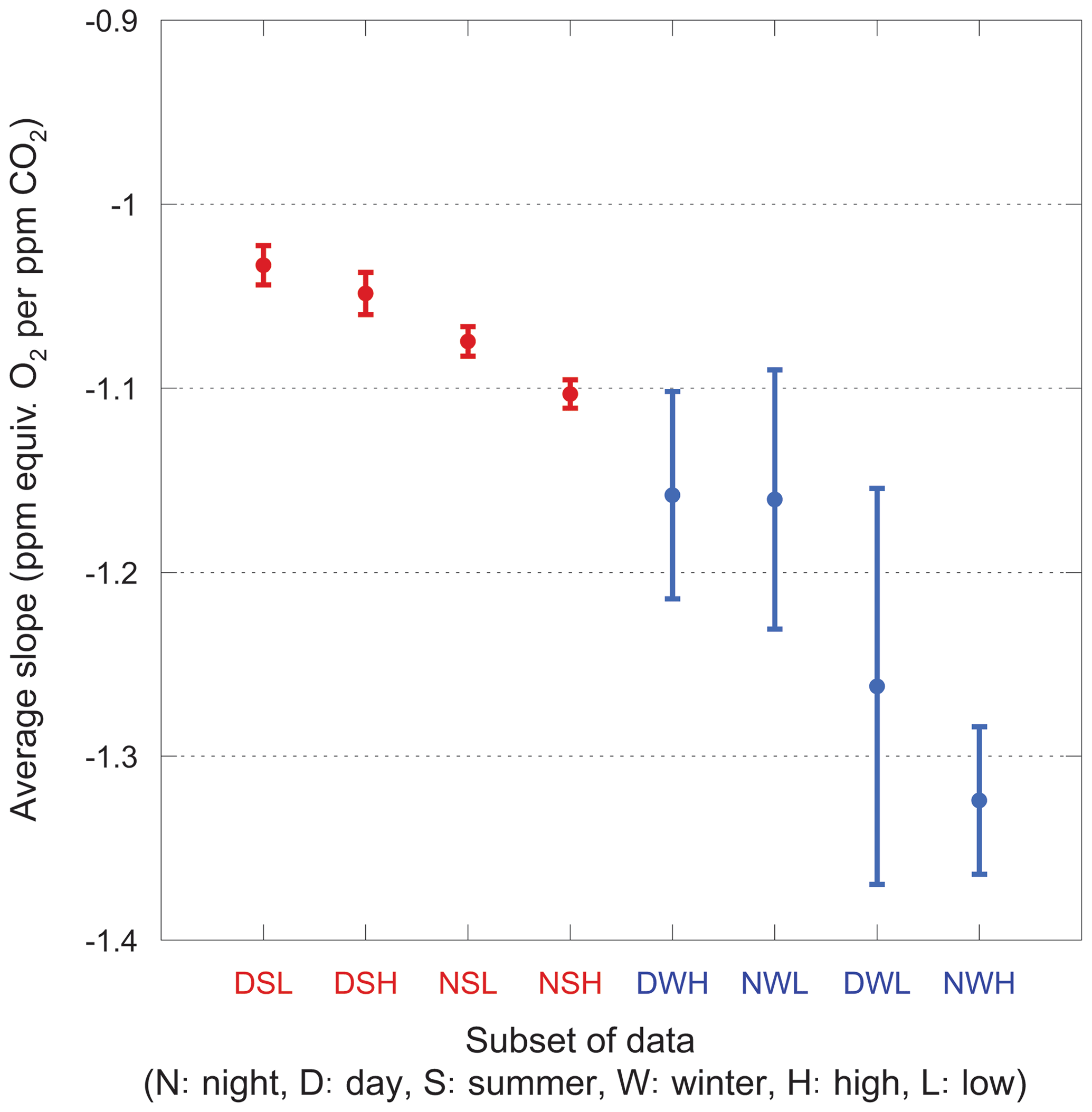
Figure 9Average slopes for various nonoverlapping subsets of the data. Error bars show the standard error on the mean. Winter data are shown in blue, summer in red. Categories are ordered by increasingly negative mean values for convenience.
The most striking feature of this plot is the large scatter in the winter data. Even with the 2.5σ iterative cut, the slopes within a category range widely and are difficult to interpret. In contrast, the summer data comprise much tighter groups and have well-defined mean values, showing the same day–night and high–low relationships as the full dataset.
Explaining these patterns is challenging. Possible factors determining the observed slope include the magnitudes of the fluxes, the dynamics of the atmosphere, and variation in the biospheric exchange ratio over time.
5.1.1 The relative size of fluxes
The relative weighting for combustion and biogenic influence in the slope will depend in part on the magnitudes of the respective fluxes across the region. Our best estimate of combustion fluxes comes from Sargent et al. (2018), who use an inverse analysis of CO2 concentration data to infer a value of 0.8 kg C m−2 yr−1 (i.e., 2.4 ) for Boston and its suburbs. We can relate this to Harvard Forest using the ACES high-resolution emission inventory developed specifically for the northeastern US (Gately and Hutyra, 2017). ACES shows a strong decrease in anthropogenic emissions moving from Boston to Harvard Forest and beyond to the west and north, with the area around the tower showing annual mean emissions closer to 0.3 .
For the biogenic fluxes, we use eddy-flux measurements of net ecosystem exchange (NEE) at Harvard Forest (Munger and Wofsy, 2017). In the summer, the daytime mean NEE at Harvard Forest is of the order of 10 or 20 for coniferous and deciduous forest, respectively, and around 5 at night. Winter NEE averages range from 2 to 3 .
Collectively, these data show the regionally averaged biogenic influence on CO2 (and by extension O2) is substantially larger than the fossil fuel source during the growing season, and dwarfs it during daytime. In winter months, anthropogenic CO2 emissions have, at most, a magnitude comparable to the biogenic flux. Further evidence that combustion sources are a minor player at Harvard Forest during the growing season comes from the observation by Potosnak et al. (1999) that CO2 and CO are correlated in winter but not summer. Finally, we note that the modeling work of Gerbig et al. (2006) showing short-term variability in CO2 is dominated by the predicted influence of vegetation.
While the U.S. EPA's inventory (Agency, 2017) shows that the primary upwind sector (west-northwest) (Moody et al., 1998) is essentially free of power plants for 100 km or more, because we lack contemporaneous measurements of CO (a tracer of combustion), it remains a possibility that plumes of power plant exhaust might occasionally influence our measurements.
In summary, based on the estimated magnitudes of the biotic and combustion fluxes, we expect the summer daytime observations of the O2:CO2 slopes to be most strongly linked to the LBER. Furthermore, the link between winter variability in CO2 and CO observed by Potosnak et al. (1999) offers one possible explanation for the much greater scatter we see in our winter data.
Comparing day and night data, fossil fuel influence may be more apparent at night when biotic fluxes are reduced (Munger and Wofsy, 2017) but fossil fuel combustion falls only slightly (Bergeron and Strachan, 2011; Velasco and Roth, 2010; Ward et al., 2015).
5.1.2 Atmospheric dynamics
With the diel cycle of insolation, the planetary boundary layer cycles between nocturnal stability and diurnal convective overturning. This is clearly evident in the climatological diel cycle of u* at Harvard Forest (Munger and Wofsy, 2017). Based on these data, we defined our 6 h daytime period to capture full photosynthetic activity and maximal vertical mixing, while our night interval captures pure respiration and maximal stratification. These dynamics suggest that air at both of our intakes would be closer in composition to air aloft during the middle of the day. Thus, daytime slopes might show more influence from distant fluxes including more fossil fuel combustion (and thus be more negative).
In addition, we expect nocturnal stability to trap fluxes from soil respiration close to the ground, amplifying their impact, particularly on the lower intake (Munger, 1996; Urbanski et al., 2007). This will lead to biologically dominated nocturnal slopes. Assuming the respiration-driven slope is closer to −1.0 than fossil fuel, we would expect to find the least negative slopes at night.
The fact that we see less negative slopes during the day than at night ( vs. ) suggests that either other factors are more important (Sect. 5.1.1 and 5.1.3) or this picture of atmospheric motion is oversimplified.
Another implication of diurnal convection and nocturnal stratification would be similar behavior of the high and low intakes during daylight hours and greater differences at night. We do see a suggestion of this in our summer data, when the high–low difference appears to be smaller during the day ( vs. ), but uncertainties are substantial. We also expect any differences driven by stratification to be reduced during the winter. Unfortunately, our winter data are too variable to meaningfully test this expectation ( and ).
Yet another possibility is a daytime temperature inversion within the forest canopy. This arises because air is warmed from above by incoming sunlight striking leaves (Jacobs et al., 1992). However, profiles of CO2 and O2 on the tower show that at Harvard Forest these inversions are often eroded by gusts from above penetrating the canopy and usually only persist in the first meter or two above ground level.
Regardless of time of day or year, velocities within the canopy will be frictionally reduced. This might suggest an enhancement of local signals (presumably with less fossil influence and thus less negative slopes) on the lower intake. This is very much consistent with our observations: with the 3σ cut, low and high slopes are and , respectively. Results are very similar to the 2.5σ cut.
Finally, we note that u* varies seasonally as well as daily. Not only is u* roughly twice as high in the winter as the summer, but it is far more variable. This may explain why the slopes in the winter months exhibit so much variation.
5.1.3 Possible variation in the biotic exchange ratio
Another possible driver of variability in slopes is variation in the biotic exchange ratio over time. For example, nocturnal plant respiration might consume molecules richer in nitrogen with higher oxidative ratios than the molecules being produced during photosynthesis (Severinghaus, 1995). Even in the complete absence of dynamical influences or fossil fuel contamination, this would lead to more negative slopes at night.
This scenario is built on a violation of mass balance that cannot persist indefinitely. Eventually, the nitrogen-poor material that was synthesized aboveground must also be respired, changing atmospheric O2 and CO2 with slopes closer to −1.0.
The viability of this explanation for our more negative nocturnal slopes becomes a question of equilibrium. In illustrative (and highly simplified) terms: is the forest as a whole out of balance, engaged in a long-term accumulation of nitrogen-poor, refractory trunk wood and a steady diversion of nitrogen into labile leaves and rootlets? Or is the forest in balance, with as many tree trunks being decomposed as are being synthesized?
Evidence pointing to a balanced forest is the isotopic measurements by Wehr and Saleska (2015) and Wehr et al. (2016), which suggest much of Harvard Forest's respired carbon was assimilated no more than a week or two earlier. Conversely, Trumbore (2000) used radiocarbon measurements to show that the mean age of respired soil carbon is 3 years. These two studies are not entirely incompatible if Trumbore's mean age is comprised of, for example, 60 % very young carbon with the balance coming from much older pools.
At this point, we are not in a position to say whether the day–night difference in slopes is due to a forest that is out of equilibrium, or whether we are measuring respiration of the full range of substrates and something else is responsible for the day–night difference in slopes.
5.2 Temporal variability in slopes
Our data are sufficiently abundant that we can examine the values of slopes as a function of time on both interannual and seasonal timescales. Figure 10 shows that one year looks much like the next, but stacked years reveal a seasonal variation in the slopes.

Figure 10(a) Slopes (averaged weekly) for a climatological year. (b) Slopes (averaged monthly) for the entire period of study. The gray line in (a) is a locally weighted least-squares fit with 46 % smoothing. It is simply intended as an objective guide to the eye.
The seasonal cycle in slopes may be due to seasonal changes in LBER itself. Trees synthesize many different compounds throughout the year (Seibt et al., 2004), each with their own oxidative ratios (Bloom et al., 1989). However, direct measurements of leaves and tree rings indicate oxidative ratios in these tissues appear invariant through the year (Gallagher et al., 2017).
Conversely, the total amount of biological activity unquestionably varies seasonally, while the fossil fuel contribution remains roughly constant. As mentioned above, earlier work at Harvard Forest using carbon monoxide and acetylene (Potosnak et al., 1999) shows clearly that fossil fuel combustion is a driver of CO2 variability in the winter, but is overwhelmed by biotic signals during the summer. Thus, the simple seasonal shift in the biotic–fossil fuel balance is a likely explanation for some, if not all, of the seasonal cycle in slopes.
Spectral analysis (using Lomb–Scargle periodograms to accommodate our irregularly spaced data; Press et al., 2007) of various subsets of the data shows some evidence of the seasonal cycle mentioned above. It appears to be mostly in the night–high-intake subset. There is also a suggestion of multi-year variation (0.6 cycles per year) in the day–low dataset and 3-week periodicity in the day–high and night–low data. Identical spectral analyses of environmental variables measured at Harvard Forest (temperature, net ecosystem exchange, ecosystem respiration, photosynthetically active radiation, and u*) all show highly significant seasonal and diel cycles, as expected.
The 3-week cycle in the day–high and night–low records is perplexing. No such cycle appears in the environmental variables listed above. Thus, our working hypothesis is that the 3-week cycles are an experimental artifact resulting from the timing of runs of calibration tanks and swapping of working tanks.
5.3 Selecting periods of heightened biogenic signal
Given the competition between biogenic and anthropogenic influences in our observations, we searched for periods when the biogenic contribution might be most dominant. We selected times when the fluxes in the immediate neighborhood were likely to dominate. Our assumption was that background variation (i.e., compositional variability due to influences beyond the ∼100 km provenance of our measurements) is likely to carry signals of continental-scale gradients with more substantial fossil fuel influences embedded therein.
One approach we considered was based on u*. We hypothesized that slopes calculated when u* was low were more likely to be biogenic since the air at our intakes was exchanging minimally with the overlying boundary layer. However, a scatter plot of slopes as a function of u* showed no correlation. Similarly, slope values were insensitive to discrete cuts on average u* (<40 cm s−1), maximum u* (<50 cm s−1), and the scatter in u* ( cm s−1).
We also explored the possibility of a link between slopes and the ranges of CO2 and O2 during the 6 h periods. Again, no correlation was apparent, whether with discrete cuts during summer and winter periods separately, or with scatter plots of slope vs. range.
We tested the hypothesis that summer periods of extended high barometric pressure with languid anticyclonic circulation might be dominated by local fluxes. Again, we observed no correlation between slope and barometric pressure, whether with discrete cuts or with scatter plots.
Finally, we looked for correlations between slopes and wind speed, direction, and variability. We found none, even when winds were from the relatively polluted sector to the southwest.
In short, relatively simple indicators of reduced advective transport show no correlation with shallower slopes. This insensitivity of our result adds support for our model of a geographically modest footprint comprised of a landscape in which biogenic fluxes are much stronger than anthropogenic ones.
Having measured changes in atmospheric CO2 and O2 in a mixed deciduous, midlatitude forest with a precision of a few micromoles per mole, we find that these species covary with an all-data average molar ratio over 6 h periods of (O2:CO2). In the absence of fossil fuel influences, our measured ratios reflect the local signature of photosynthesis and respiration (LBER). If our data represent a mix of forest and fossil fuel fluxes, −1.081 is a lower (most negative) limit on LBER. Adopting a two-end-member mixing model, the best value would be taken from the subset of the data with the smallest fossil fuel contribution and presumably the shallowest measured slope. Restricting our dataset to daytime values from the low intake in summer (when we expect local influences to be maximal due to vigorous biotic activity and modest coupling with the air above the canopy), we find a slope of .
Our values are consistent with measurements in other temperate forests. The consistency of elemental ratios in the work of Worrall et al. (2013) across a range of study sites suggests the Harvard Forest result may have broad applicability. Furthermore, basic constraints in plant physiology argue against wildly divergent values across species (Björkman and Demmig, 1987). Nonetheless, similar studies at other sites are required before concluding a value very close to 1.0 is globally representative.
Also, it is still possible that gross photosynthetic and respiratory exchanges could exhibit O2:CO2 ratios individually that differ from the (much smaller) net uptake of CO2 and release of O2. For this reason it is important to track O2 in process-based ecosystem models, enabling predictions of both LBER and αB while matching observations.
Even with this qualification, our measurements provide valuable insight into the nature of O2 and CO2 exchange in a temperate forest. They also suggest that the best value for αB in calculations partitioning global carbon fluxes may be lower than 1.1, the value widely used to date (Keeling and Manning, 2014). At the least, studies that rely on αB should explore sensitivity to values as low as 1.0.
If our results do indeed match the ratio of the global net carbon sink, the use of 1.03 for αB leads to a 7 % increase in terrestrial carbon uptake and an equivalent reduction in oceanic carbon storage (see Eq. 8 of Keeling and Manning, 2014). While this adjustment is within the uncertainties on these terms in the global carbon budget, it would nonetheless be an important correction.
All of the data presented in this study can be found in the Harvard Forest Data Archive as dataset HF306 (Battle and Munger, 2018).
MB conceived of the experiment. MB built and operated the hardware and wrote software with assistance from JWM, ES, RP, RH, ZD, JS, JW, KG, SS, JC and SD. MB and MC performed data analysis. MB wrote the paper with assistance from JWM and MC.
The authors declare that they have no conflict of interest.
This article is part of the special issue “The 10th International Carbon Dioxide Conference (ICDC10) and the 19th WMO/IAEA Meeting on Carbon Dioxide, other Greenhouse Gases and Related Measurement Techniques (GGMT-2017) (AMT/ACP/BG/CP/ESD inter-journal SI)”. It is a result of the 10th International Carbon Dioxide Conference, Interlaken, Switzerland, 21–25 August 2017.
Analysis of our data was greatly aided by a suggestion from Alessandro Cescatti. We also thank Maryann Sargent and Richard Wehr for helpful conversations and Taylor Jones for sharing code. Robert Stevens helped with machining, Dj Merrill provided computing support, and Emery Boose and John Budney gave invaluable assistance at Harvard Forest.
We thank Britton Stephens and the anonymous reviewer for exceptionally thoughtful reviews and suggestions that greatly improved the paper.
Operation of the Harvard Forest flux tower site is supported by the AmeriFlux Management Project with funding by the U.S. Department of Energy's Office of Science under contract no. DE-AC02-05CH11231, and additionally as a part of the Harvard Forest LTER site supported by the National Science Foundation (DEB-1237491). Support for the tower operation during the period examined here, as well as partial support for the O2−CO2 sampling equipment, came from the U.S. Dept of Energy Office of Science through programs that are no longer active (including the National Institute of Global Environmental Change and the National Institute for Climate Change Research). Further support for the sampling equipment was provided by Bowdoin College.
This paper was edited by Nicolas Gruber and reviewed by Britton Stephens and one anonymous referee.
Agency, U. S. E. P.: Greenhouse Gas Reporting Program, available at: https://www.epa.gov/ghgreporting (last access: 28 April 2019), 2017. a
Battle, M. and Munger, W.: Atmospheric Oxygen and Carbon Dioxide at Harvard Forest EMS Tower since 2006, Harvard Forest Data Archive, HF306, available at: http://harvardforest.fas.harvard.edu:8080/exist/apps/datasets/showData.html?id=hf306 (last access: 16 June 2019), 2018. a
Bergeron, O. and Strachan, I. B.: CO2 sources and sinks in urban and suburban areas of a northern mid-latitude city, Atmos. Environ., 45, 1564–1573, 2011. a, b, c
Björkman, O. and Demmig, B.: Photon yield of O2 evolution and chlorophyll flourescence characteristics at 77 K among vascular plants of diverse origins, Planta, 170, 489–504, https://doi.org/10.1007/BF00402983, 1987. a
Blaine, T. W., Keeling, R. F., and Paplawsky, W. J.: An improved inlet for precisely measuring the atmospheric Ar∕N2 ratio, Atmos. Chem. Phys., 6, 1181–1184, https://doi.org/10.5194/acp-6-1181-2006, 2006. a
Bloom, A., Caldwell, R., Finazzo, J., Warner, R., and Weissbart, J.: Oxygen and carbon dioxide fluxes from barley shoots depend on nitrate assimilation, Plant Physiol., 91, 352–356, 1989. a, b
Conley, M. M.: Using atmopsheric O2 and CO2 to determine the stoichiometry of photosynthesis and respiration in a temperate forest, Bachelor of Arts thesis, Bowdoin College, available at: https://digitalcommons.bowdoin.edu/honorsprojects/87/ (last access: 21 June 2019), 2018. a
Deming, W. E.: Statistical adjustment of data, Dover Publications, New York, 2011. a
Gallagher, M. E., Liljestrand, F. L., Hockaday, W. C., and Masiello, C. A.: Plant species, not climate, controls aboveground biomass O2:CO2 exchange ratios in deciduous and coniferous ecosystems, J. Geophys. Res.-Biogeo., 122, 2314–2324, 2017. a, b
Gately, C. K. and Hutyra, L. R.: Large Uncertainties in Urban-Scale Carbon Emissions, J. Geophys. Res.-Atmos., 122, 11242–11260, 2017. a
Gerbig, C., Lin, J. C., Munger, J. W., and Wofsy, S. C.: What can tracer observations in the continental boundary layer tell us about surface-atmosphere fluxes?, Atmos. Chem. Phys., 6, 539–554, https://doi.org/10.5194/acp-6-539-2006, 2006. a, b, c, d
Hall, B.: Calculation of expanded uncertainties for CO2, available at: https://www.esrl.noaa.gov/gmd/ccl/ccl_uncertainties_co2.html (last access: 4 April 2019), 2017. a
Hockaday, W., Masiello, C., Randerson, J., Smernik, R., Baldock, J., Chadwick, O., and Harden, J.: Measurement of soil carbon oxidation state and oxidative ratio by 13C nuclear magnetic resonance, J. Geophys. Res., 114, G02014, https://doi.org/10.1029/2008JG000803, 2009. a
Jacobs, A. F. G., van Boxel, J. H., and Shaw, R. H.: The dependence of canopy layer turbulence on within-canopy thermal stratification, Agr. Forest Meteorol., 58, 247–256, 1992. a
Keeling, R. and Manning, A.: Studies of Recent Changes in Atmospheric O2 Content, in: Treatise on Geochemistry, 2 edn., Elsevier Inc., 5, 385–404, https://doi.org/10.1016/B978-0-08-095975-7.00420-4, 2014. a, b, c, d, e
Keeling, R., Manning, A., McEvoy, E., and Shertz, S.: Methods for measuring changes in atmospheric O2 concentration and their application in southern hemisphere air, J. Geophys. Res., 103, 3381–3397, 1998. a, b, c
Keeling, R., Paplawsky, W., and Cox, A.: On the long-term stability of reference gases for atmospheric O2∕N2 and CO2 measurements, Tellus B, 59, 3–14, 2007. a
Keeling, R. F.: Development of an Interferometric Oxygen Analyzer for Precise Measurement of the Atmospheric O2 Mole Fraction, PhD thesis, Harvard University, available at: http://bluemoon.ucsd.edu/publications/ralph/34_PhDthesis.pdf (last access: 5 May 2018), 1988. a
Keeling, R. F. and Shertz, S. R.: Seasonal and interannual variations in atmospheric oxygen and implications for the global carbon cycle, Nature, 358, 723–727, 1992. a, b
Keeling, R. F., Blaine, T., Paplawsky, B., Katz, L., Atwood, C., and Brockwell, T.: Measurments of changes in atmospheric Ar∕N2 ratio using a rapid-switching, single-capillary mass spectrometer system, Tellus B, 56, 322–338, 2004. a
Masiello, C., Gallagher, M., Randerson, J., Deco, R., and Chadwick, O.: Evaluating two experimental approaches for measuring ecosystem carbon oxidation state and oxidative ratio, J. Geophys. Res., 113, G03010, https://doi.org/10.1029/2007JG000534, 2008. a
Moody, J., Munger, J., Goldstein, A., Jacobs, D., and Wofsy, S.: Harvard Forest regional-scale air mass composition by Patterns in Atmospheric Transport History (PATH), J. Geophys. Res., 103, 13181–13194, 1998. a
Munger, J. W.: Atmospheric deposition of reactive nitrogen oxides and ozone in a temperate deciduous forest and a subarctic woodland: 1. Measurements and mechanisms, J. Geophys. Res., 101, 12639–12657, 1996. a
Munger, W. and Wofsy, S.: Canopy-Atmosphere Exchange of Carbon, Water and Energy at Harvard Forest EMS Tower since 1991, Harvard Forest Data Archive: HF004, available at: http://harvardforest.fas.harvard.edu:8080/exist/apps/datasets/showData.html?id=hf004 (last access: 16 June 2019), 2017. a, b, c, d, e
NOAA: HYSPLIT – Hybrid Single Particle Lagrangian Integrated Trajectory model, available at: https://ready.arl.noaa.gov/HYSPLIT.php, last access: 2 April 2018. a, b
Potosnak, M. J., Wofsy, S. C., Denning, A. S., Conway, T. J., Munger, J. W., and Barnes, D. H.: Influence of biotic exchange and combustion sources on atmospheric CO2 concentrations in New England from observations at a forest flux tower, J. Geophys. Res., 104, 9561–9569, 1999. a, b, c
Press, W. H., Teukolsky, S. A., Vetterling, W. T., and Flannery, B. P.: 13.8 Spectral Analysis of Unevenly Sampled Data, in: Numerical Recipes: The Art of Scientific Computing, 3rd edn., Cambridge University Press, Cambridge, 685–692, 2007. a
Randerson, J., Masiello, C., Still, C., Rahn, T., Poorter, H., and Field, C.: Is carbon within the global terrestrial biosphere becoming more oxidized? Implications for trends in atmopsheric O2, Glob. Change Biol., 12, 260–271, https://doi.org/10.1111/j.1365-2486.2006.01099.x, 2006. a
Sargent, M., Barrera, Y., Nehrkorn, T., Hutyra, L., Gately, C., Jones, T., McKain, K., Sweeney, C., Hegarty, J., Hardiman, B., and Wofsy, S.: Anthropogenic and Biogenic CO2 fluxes in the Boston urban region, P. Natl. Acad. Sci. USA, 115, 7491–7496, 2018. a
Seibt, U., Brand, W., Heimann, M., Lloyd, J., Severinghaus, J., and Wingate, L.: Observations of O2:CO2 exchange ratios during ecosystem gas exchange, Global Biogeochem. Cy., 18, 1–18, https://doi.org/10.1029/2004GB002242, 2004. a, b
Severinghaus, J. P.: Studies of the Terrestrial O2 and Carbon Cycles in Sand Dune Gases and in Biosphere 2, PhD thesis, Columbia University, 1995. a, b, c
Steinbach, J., Gerbig, C., Rödenbeck, C., Karstens, U., Minejima, C., and Mukai, H.: The CO2 release and Oxygen uptake from Fossil Fuel Emission Estimate (COFFEE) dataset: effects from varying oxidative ratios, Atmos. Chem. Phys., 11, 6855–6870, https://doi.org/10.5194/acp-11-6855-2011, 2011. a
Stephens, B., Bakwin, P., Tans, P., Teclaw, R., and Baumann, D.: Application of a differential fuel-cell analyzer for measuring atmospheric oxygen variations, J. Atmos. Ocean. Tech., 24, 82–94, https://doi.org/10.1175/JTECH1959.1, 2007. a, b, c, d, e, f
Sturm, P., Leuenberger, M., and Schmidt, M.: Atmospheric O2, CO2 and δ13C observations from the remote sites Jungfraujoch, Switzerland, and Puy de Dô̂me, France, Geophys. Res. Lett., 32, L17811, https://doi.org/10.1029/2005GL023304, 2005. a
Trumbore, S.: Age of Soil Organic Matter and Soil Respiration: Radiocarbon Constraints on Belowground C Dynamics, Ecol. Appl., 10, 399–411, 2000. a
Urbanski, S. P., Barford, C. C., Wofsy, S. C., Kucharik, C. J., Pyle, E. H., Budney, J., McKain, K., Fitzjarrald, D. R., Czikowsky, M. J., and Munger, J. W.: Factors controlling CO2 exchange on time scales from hourly to decadal at Harvard Forest, J. Geophys. Res., 112, G02020, https://doi.org/10.1029/2006JG000293, 2007. a, b, c
Velasco, E. and Roth, M.: Cities as net sources of CO2: Review of atmospheric CO2 exchange in urban environments measured by eddy covariance technique, Geography Compass, 4, 1238–1259, 2010. a, b
Ward, H. C., Kotthaus, S., Grimmond, C. S. B., Bjorkegren, A., Wilkinson, M., Morrison, W. T. J., Evans, J. G., Morison, J. I. L., and Iamarino, M.: Effects of urban density on carbon dioxide exchanges: Observations of dense urban, suburban and woodland areas of southern England, Environ. Pollut., 198, 186–200, 2015. a, b
Wehr, R. and Saleska, S.: An improved isotopic method for partitioning net ecosystem-atmosphere CO2 exchange, Agr. Forest Meteorol., 214–215, 515–531, 2015. a
Wehr, R., Munger, J., McManus, J., Nelson, D., Zahniser, M., Davidson, E., Wofsy, S., and Saleska, S.: Seasonality of temperate forest photosynthesis and daytime respiration, Nature, 534, 680–683, https://doi.org/10.1038/nature17966, 2016. a
Worrall, F., Clay, G. D., Masiello, C. A., and Mynheer, G.: Estimating the oxidative ratio of the global terrestrial biosphere carbon, Biogeochemistry, 115, 23–32, 2013. a, b, c
Zhao, C. and Tans, P.: Estimating uncertainty of the WMO mole fraction scale for carbon dioxide in air, J. Geophys. Res., 111, D08S09, https://doi.org/10.1029/2005JD006003, 2006. a
- Abstract
- Introduction
- Methods
- Observations
- The relationship between local O2:CO2 ratios and the local biotic exchange ratio (LBER)
- Discussion of observations
- Conclusions
- Data availability
- Author contributions
- Competing interests
- Special issue statement
- Acknowledgements
- Financial support
- Review statement
- References