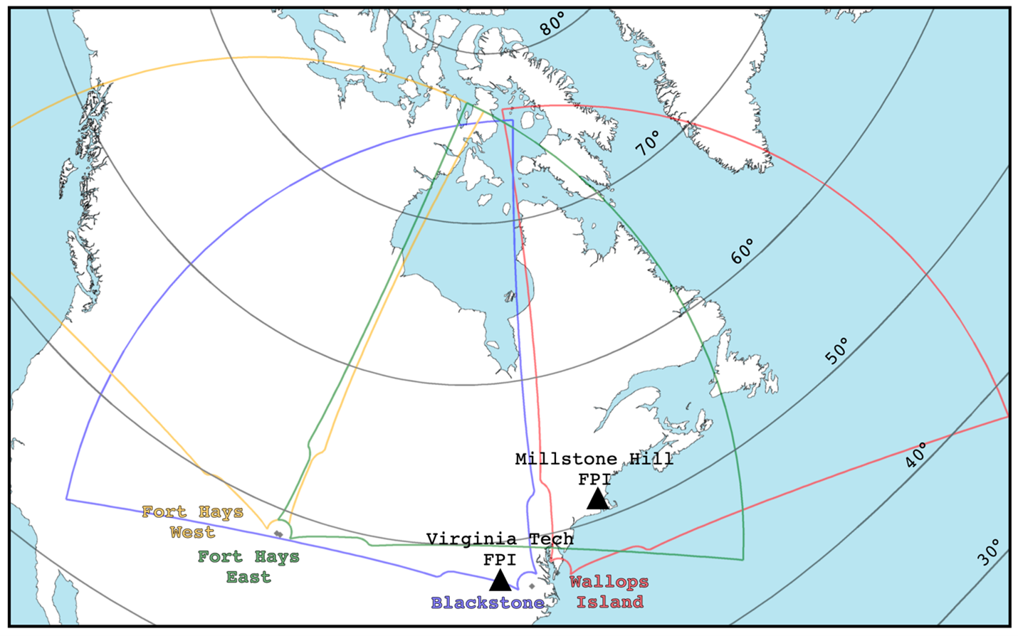
Figure 1: The fields of view of the Fort Hays West (yellow), Fort Hays East (green), Blackstone (blue), and Wallops Island (red) SuperDARN radars. Also shown are the locations of two FPIs (black triangles), with one at Millstone Hill Geospace Facility and the other at Virginia Tech (November 2013). Black lines indicate parallels of constant altitude-adjustment-corrected geomagnetic (AACGM) latitude (Figure obtained from Billett et al., 2022).
The upper atmosphere of Earth is constantly being impacted by the flow of charged particles being released from the sun. This flow (the solar wind) carries with it a magnetic field which distorts and reshapes that of Earth, ultimately resulting in a large amount of electromagnetic space weather energy being channelled into the polar regions. One of the most frequently observed outcomes of this process is the Dungey cycle [Dungey, 1961], which is where the bulk ionised population of upper atmosphere (the ionosphere) forms a large circulation pattern spanning thousands of kilometres across Earth’s poles. However, a much less understood process is how those ions affect the neutral part of the atmosphere (the thermosphere), the dynamics of which can have severe impacts on satellite-based infrastructure (for example, during the “SpaceX destruction event” in early 2022). Even less characterised is the impact of space weather at latitudes below the poles, made difficult due to the infrequency of events which could cause such a large disturbance, as well as the challenges in obtaining thermospheric measurements.
In a recent study [Billett et al., 2022], winds in the thermosphere above North America were observed under the influence of sub-auroral polarisation streams [SAPS; Foster and Burke, 2002]. SAPS are an uncommon feature of the mid-latitude ionosphere which consist of fast flows distinctly detached from the high-latitude Dungey cycle circulation. The winds were obtained from two cameras, at Virginia Tech University and Millstone Hill Observatory, known as Fabry-Perot Interferometers (FPIs). FPIs get thermospheric winds by measuring the doppler shift of nightglow and aurora, but that means their primary limitation is that they can only operate under clear skies and in complete darkness. Simultaneous wind measurements from two FPI’s separated by a few hundred kilometres, coupled with a SAPS event, thus offered a unique and rare opportunity to get insights into the effects of space weather on the mid-latitude atmosphere.
To measure the SAPS in this study, 4 high-frequency radars which are part of the Super Dual Auroral Radar Network [SuperDARN; Greenwald et al., 1995] were used to measure the line-of-sight ionospheric plasma velocity. A diagram showing the fields-of-view of the SuperDARN radars (Fort Hays West, Fort Hays East, Blackstone, and Wallops Island) and FPIs (Virginia Tech and Millstone Hill) used is shown in Figure 1, with latitude parallels in geomagnetic coordinates. For reference, the lower latitude of the auroral oval during the SAPS event was consistently around 60°, meaning the FPIs and a large portion of the SuperDARN radar FOVs were observing the sub-auroral atmosphere.
Figure 2 shows an overview of the event in polar format, magnetic latitude – magnetic local time coordinates, which took place on the 9th November, 2013. 6 panels of data are shown, one hour apart, showing the line-of-sight plasma velocities measured by the SuperDARN radars (colours) and thermospheric disturbance wind vectors measured by the FPI’s (black arrows). The red circle shows the approximate lower boundary of the auroral oval determined by the SSUSI instrument on board DMSP F-16, F-17, and F-18 [Paxton et al., 2002]. The SAPS in Figure 2 are characterised by fast plasma drifts measured by the SuperDARN radars in the westward direction (clockwise around the circular plot) below the auroral oval, which are displayed as either yellow-red (away from the radar site) or green-blue (towards).
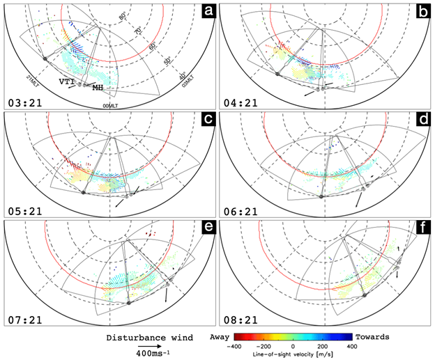
Figure 2: Nightside polar plots of plasma velocity data from four SuperDARN radars and disturbance neutral wind velocity vectors from the VTI and MH FPIs (black arrows) for times on 9 November 2013. The red circle is the approximate location of the auroral oval lower-latitude boundary, derived from Special Sensor Ultraviolet Spectrographic Imager (SSUSI) data aboard whichever Defense Meteorological Satellite Program (DMSP) instrument (F-16, F-17, or F-18) last crossed the pole. The VTI FPI is the arrow with a base at a slightly lower latitude compared to the MH FPI (Figure obtained from Billett et al., 2022).
The SAPS flows and disturbance winds in Figure 2 both reach several hundred metres per second. However, the differences between the two wind measurements at Virginia Tech (VTI) and Millstone Hill (MH) sheds light onto the how the ionosphere and thermosphere interact with each other at these different locations. For example, winds at MH and VTI accelerate westward (clockwise) and equatorward (towards the outside of the circular plots) respectively, but the MH winds slow down at 06:21 and even turn eastward (anti-clockwise) at 08:21. This implies the forces acting on the thermosphere, driven by the SAPS, are significantly different at both locations, even though they are relatively close spatially.
The three biggest forces which act on thermospheric winds are ion-drag, pressure gradients, and Coriolis. The Ion-drag force is the exchange of momentum when ionised and neutral particles collide. Pressure gradient forces are set up when a region of the thermosphere is heated, such as from direct solar extreme ultra-violet radiation, which causes winds to flow in the direction of cooler and less dense space. Finally, the Coriolis force is inertial and acts on neutral particles which are moving at a velocity that is differential to the Earth’s rotation. We know that at both FPI sites during the SAPS event shown above, the balance of these forces was different because the winds were different. But how do we know what forces are important at each location?
The impacts of pressure gradient forces are apparent across the entire thermosphere. In fact, the dominant motion of thermospheric winds is from the dayside to the nightside because of constant solar heating of local times situated in daylight. SAPS can also cause pressure gradients via Joule heating, which is the left-over energy released into the ionosphere after work has been done moving the plasma itself. The SAPS in Figure 2, from 03:21 to 05:21, cause an equatorward pressure gradient force and so the winds accelerate equatorward, particularly at VTI which is directly adjacent to the SAPS region. The Coriolis force then kicks in, causing the equatorward winds to rotate slightly westward.
At MH there is a slightly different story however, as the winds there act more westward, in the same direction as the motion of the SAPS in Figure 2. This implies that thermospheric winds above MH are more significantly impacted by ion-drag instead of pressure gradients. As Millstone Hill is at a higher latitude than Virginia Tech, it was located directly in the vicinity of the SAPS instead of adjacent to it. Therefore, the motion of the ionospheric plasma was having a much more direct control on the motion of the thermospheric neutrals at MH than at VTI. As a result, winds at the two locations experienced very different responses to the same ionospheric phenomenon.
Overall, the study summarised here and presented in more detail in Annales Geophysicae shows how dynamic the Earth’s upper atmosphere is under relatively small spatial scales. Because thermospheric winds are significantly more difficult to measure in comparison to ionospheric flows, there is much we still do not known about how the two are coupled. Ultimately, this means there is a lot of uncertainty in our understanding of how electromagnetic energy from space weather events is deposited and utilised in the atmosphere. As SpaceX showed earlier this year, these uncertainties can propagate into very costly problems.
References
[1] J. W. Dungey, 1961, Phys. Rev. Lett. 6, 47 (https://doi.org/10.1103/PhysRevLett.6.47)
[2] S.Gorman, 2022, Reuters (https://www.reuters.com/lifestyle/science/solar-storm-disables-40-newly-launched-spacex-satellites-2022-02-09/)
[3] D. D. Billett, et al., 2022, Ann. Geophys., 40, 571–583, 2022 (https://doi.org/10.5194/angeo-40-571-2022)
[4] J. C. Foster, W. J. Burke, 2011, Eos Trans. AGU, 83( 36), 393– 394, (https://doi.org/10.1029/2002EO000289)
[5] R. A. Greenwald, et al., 1995, Space Sci Rev 71, 761–796 (https://doi.org/10.1007/BF00751350)
[6] L. J. Paxton et al., 2002, Proc. SPIE 4485, Optical Spectroscopic Techniques, Remote Sensing, and Instrumentation for Atmospheric and Space Research IV, (https://doi.org/10.1117/12.454268)