Name of proxy
Fluctuations of mountain glaciers
Type of record
Geomorphological features
Paleoenvironment
Continent – High mountain areas
Period of time investigated
From historical periods (c.a. 300 years ago) to the end of the Pleistocene (up to 200 000 years back in time)
How does it work?
Mountain – or “alpine” – glaciers are small ice bodies (from 1 to 10 000 km2). Although they represent only 0.3% of the total volume of the present-day cryosphere, they contain a large amount of useful information on the past climatic conditions on the continents. The position of the glacier margins, and its volume, is defined by its mass balance (the balance between ice accumulation and ice melt), that is mainly controlled by two important climate variables: air temperature and snow precipitation. Their internal behaviour is very sensitive to climate change, and they respond rapidly (<50 years) to climatic fluctuations. This gives alpine glaciers the ability to record climate change with a high temporal resolution.
The peculiarity of this climatic proxy is that it brings together several fields of research: glaciology, geomorphology, geochronology, and numerical modeling. In order to interpret mountain glacier fluctuations as climatic proxies, it is necessary to:
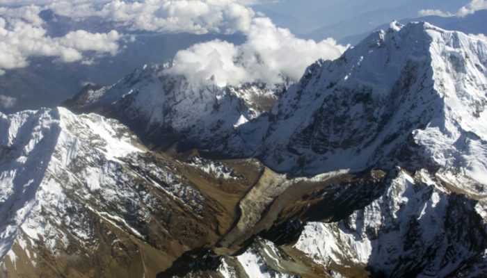
(i) Observe and interpret past glaciated landscapes (including landforms such as moraines and roches moutonnées) to infer past mass balances. This task often requires several days of field work in remote high area locations (Fig. 1a);
(ii) Establish the age of formation of these landscapes, most of the time using carbon-14, or other rare isotopes (such as beryllium-10 or helium-3). The concentrations of these rare isotopes increases with the time spent by a rock at the surface (Fig. 1b);
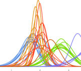
(iii) Perform computer-based numerical model simulations to infer the main climatic parameters (temperatures and precipitation) from the variations of glacial volumes (Fig. 1c).
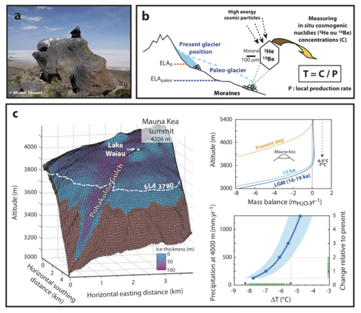
Figure 1: Summary of the methodology used to derive paleoclimatic conditions from the fluctuations of mountain glaciers a) Sampling of a boulder sitting on a moraine for surface exposure dating using cosmogenic helium-3 (Altiplano, Tropical Andes), b) Principles of dating using in situ cosmogenic nuclides, c) Numerical modeling to interpret past glacial extent in paleotemperatures and paleoprecipitation conditions (from Blard et al., 2007)
Note that the position of a glacier may be considered as a “2 unknowns – 1 equation” problem, making useful any independent inputs from other continental paleoclimatic proxies, when available. These could for example be pollen-based reconstructions, lake level fluctuations or isotopic tools (measured in speleothems, lacustrine inorganic deposits or biogenic carbonates) that can bring quantitative constraints on temperature, precipitation or both (see previous posts for more information). If such complementary proxies are not available in the studied areas, it is necessary to remain cautious and propose a range of possible paleotemperature and paleoprecipitation reconstructions (Fig. 1c).
What are the key findings made using this proxy?
In some high altitude areas, Alpine glaciers, and changes in their mass balance over time, are the only indicators of paleoclimatic change. They have e.g. allowed us to understand that:
(i) The end of the Last Glacial Maximum (c.a. 18,000 years ago) was broadly synchronous (Schaefer et al., 2006; Clark et al., 2009);
(ii) The lapse rate (i.e. the vertical temperature gradient in the atmosphere – temperatures are lower higher up a mountain) was steepened during the Last Glacial Maximum (Blard et al., 2007), although this is controversial in some regions (Tripati et al., 2014);
(iii) The Little Ice Age (XVIIth-XIXth centuries) was a global event (Rabatel et al., 2006);
(iv) Because glaciers respond to both temperatures and precipitation amount, glacier fluctuations have also been used to reconstruct the changes in past precipitation or ‘paleoprecipitation’ at a high spatial resolution. The typical size of glacier watersheds is few hundreds to thousands square kilometers, which make them ideal paleorainfall gauges. This allows us to determine the paleoprecipitation variability at the regional scale (e.g. Martin, 2016 used paleoglaciers to establish the spatial pattern of rainfall in the Tropical Andes during the Heinrich 1 event, 16,000 years ago).
References
Blard et al. (2007) - Persistence of full glacial conditions in the central Pacific until 15,000 years ago, Nature 449 (7162), 591.

Clark et al. (2009) - The last glacial maximum, Science 325 (5941), 710-714.

Martin, PhD Thesis, Université de Lorraine, 2016

Rabatel et al. (2006) - Glacier recession on Cerro Charquini (16 S), Bolivia, since the maximum of the Little Ice Age (17th century), Journal of Glaciology 52 (176), 110-118.

Schaefer et al. (2006) - Near-synchronous interhemispheric termination of the last glacial maximum in mid-latitudes, Science 312 (5779), 1510-1513.

Tripati et al. (2014) - Modern and glacial tropical snowlines controlled by sea surface temperature and atmospheric mixing, Nature Geoscience 7 (3), 205-209.
Edited by the editorial board